Decoupling Conformal Predictors from Learners#
Importing packages#
In the examples below, we will be using the three main classes ConformalClassifier, ConformalRegressor, and ConformalPredictiveSystem from the crepes package, as an alternative to using the classes WrapClassifier and WrapRegressor, which tightly integrate the conformal predictor with the learner, as illustrated here. We will here see how we instead may generate conformal predictors that are decoupled from
the underlying model. In the examples, we will be using a helper class and functions from crepes.extras as well as NumPy, pandas, matplotlib and sklearn.
[1]:
import numpy as np
import pandas as pd
import matplotlib.pyplot as plt

from sklearn.ensemble import RandomForestClassifier, RandomForestRegressor
from sklearn.model_selection import train_test_split
from sklearn.datasets import fetch_openml

from scipy.stats import kstest

from crepes import (ConformalClassifier,
                    ConformalRegressor,
                    ConformalPredictiveSystem,
                    __version__)

from crepes.extras import hinge, margin, binning, DifficultyEstimator

print(f"crepes v. {__version__}")

np.random.seed(602211023)
np.set_printoptions(legacy='1.25')
crepes v. 0.9.1
Conformal classifiers (CC)#
Importing and splitting a classification dataset#
Let us import a classification dataset from www.openml.org.
[2]:
dataset = fetch_openml(name="gas-drift", parser="auto")

X = dataset.data.values.astype(float)
y = dataset.target.values
We now split the dataset into a training and a test set, and further split the training set into a proper training set and a calibration set.
[3]:
X_train, X_test, y_train, y_test = train_test_split(X, y, test_size=0.5)

X_prop_train, X_cal, y_prop_train, y_cal = train_test_split(X_train, y_train,
                                                            test_size=0.25)
Standard conformal classifier#
Let us first create and fit a random forest in the usual way (using the proper training set only):
[4]:
rf = RandomForestClassifier(n_jobs=-1, n_estimators=500)

rf.fit(X_prop_train, y_prop_train)
[4]:
RandomForestClassifier(n_estimators=500, n_jobs=-1)In a Jupyter environment, please rerun this cell to show the HTML representation or trust the notebook.
On GitHub, the HTML representation is unable to render, please try loading this page with nbviewer.org.
Parameters
| n_estimators | 500 | |
| criterion | 'gini' | |
| max_depth | None | |
| min_samples_split | 2 | |
| min_samples_leaf | 1 | |
| min_weight_fraction_leaf | 0.0 | |
| max_features | 'sqrt' | |
| max_leaf_nodes | None | |
| min_impurity_decrease | 0.0 | |
| bootstrap | True | |
| oob_score | False | |
| n_jobs | -1 | |
| random_state | None | |
| verbose | 0 | |
| warm_start | False | |
| class_weight | None | |
| ccp_alpha | 0.0 | |
| max_samples | None | |
| monotonic_cst | None |
Let us also calculate non-conformity scores for the calibration set using the hinge function imported from crepes.extras, which takes predicted probabilities, class names and labels as input:
[5]:
alphas_cal = hinge(rf.predict_proba(X_cal), rf.classes_, y_cal)
Using the non-conformity scores, we create and fit a standard conformal classifier by:
[6]:
cc_std = ConformalClassifier()

cc_std.fit(alphas_cal)

display(cc_std)
ConformalClassifier(fitted=True, mondrian=False)
In order to make predictions for a test set, we need non-conformity scores for this too; note that class names and labels should not be provided in this case:
[7]:
alphas_test = hinge(rf.predict_proba(X_test))
We obtain p-values for the test set from the non-conformity scores by:
[8]:
cc_std.predict_p(alphas_test)
[8]:
array([[7.11853998e-02, 6.81623163e-04, 7.51952414e-05, 7.22822111e-03,
        1.83551541e-03, 1.25354912e-03],
       [7.69995483e-04, 4.02198309e-01, 3.28246348e-03, 8.46337362e-04,
        1.03880711e-03, 1.29555038e-03],
       [1.65747617e-03, 1.16900791e-03, 2.02917868e-04, 5.02167131e-05,
        7.65836044e-01, 1.70578620e-03],
       ...,
       [1.30852359e-03, 1.38763636e-03, 2.20624808e-03, 4.54321090e-03,
        2.99559728e-03, 2.06218609e-01],
       [1.89321540e-03, 1.75937091e-03, 1.64400289e-03, 6.98791143e-03,
        2.22087512e-03, 1.16866012e-01],
       [2.90605130e-03, 1.94900613e-03, 1.74838116e-03, 3.30855703e-03,
        7.68918667e-02, 7.03350329e-03]])
If we want only the p-values for the correct labels, we need to provide the class names together with the labels and set all_classes=False:
[9]:
p_values = cc_std.predict_p(alphas_test, all_classes=False, classes=rf.classes_, y=y_test)
display(p_values)
array([0.06903153, 0.40886435, 0.74415504, ..., 0.20719285, 0.11680768,
       0.07797522])
Let us take a look at how the p-values are distributed. From the visual inspection they may appear be approximaly uniformly distributed; this is however not guaranteed, since the p-values are not independent (see further below for semi-online conformal classifiers, for which this indeed holds). It is hence not very surprising if the Kolmogorov-Smirnov test allows us to reject that the p-values are sampled from a uniform distribution.
[10]:
plt.ecdf(p_values)
plt.xlim(0,1)
plt.xlabel("p-value")
plt.ylabel("ECDF")
plt.show()

print(f"KS-test: {kstest(p_values, "uniform").pvalue}")
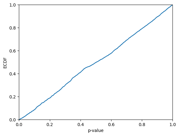
KS-test: 0.0006403345328411814
We can also obtain predictions sets, here represented by binary vectors indicating the presence (1) or absence (0) of each class label, for some specified confidence level (the default is 0.95):
[11]:
cc_std.predict_set(alphas_test, confidence=0.95)
[11]:
array([[1, 0, 0, 0, 0, 0],
       [0, 1, 0, 0, 0, 0],
       [0, 0, 0, 0, 1, 0],
       ...,
       [0, 0, 0, 0, 0, 1],
       [0, 0, 0, 0, 0, 1],
       [0, 0, 0, 0, 1, 0]])
If we intstead would like to have the prediction sets represented by lists of labels, we have to provide the label names:
[12]:
label_sets = cc_std.predict_set(alphas_test, labels=rf.classes_, confidence=0.95)
label_sets[:20]
[12]:
[['1'],
 ['2'],
 ['5'],
 ['2'],
 ['4'],
 ['6'],
 ['6'],
 ['1'],
 ['2'],
 ['6'],
 ['2'],
 ['2'],
 ['1'],
 ['2'],
 ['6'],
 [],
 [],
 ['6'],
 ['1'],
 ['5']]
We may also evaluate the predictions; here using all available metrics, which is the default:
[13]:
cc_std.evaluate(alphas_test, rf.classes_, y_test, confidence=0.95)
[13]:
{'error': 0.0404025880661395,
 'avg_c': 0.9610352264557872,
 'one_c': 0.9610352264557872,
 'empty': 0.038964773544212794,
 'ks_test': 0.0009057526555128788,
 'time_fit': 1.1920928955078125e-06,
 'time_evaluate': 0.4990394115447998}
Alternatively, we could calculate non-conformity scores using the margin function, also imported from crepes.extras, which similar to hinge, takes predicted probabilities, class names and labels as input:
[14]:
alphas_margin_cal = margin(rf.predict_proba(X_cal), rf.classes_, y_cal)
Using the new non-conformity scores, we create and fit a standard conformal classifier by:
[15]:
cc_margin_std = ConformalClassifier()

cc_margin_std.fit(alphas_margin_cal)

display(cc_margin_std)
ConformalClassifier(fitted=True, mondrian=False)
In order to make predictions for the test set, we again need the non-conformity scores for this too:
[16]:
alphas_margin_test = margin(rf.predict_proba(X_test))
Let us again evaluate the predictions:
[17]:
cc_margin_std.evaluate(alphas_margin_test, rf.classes_, y_test, confidence=0.95)
[17]:
{'error': 0.036089144500359494,
 'avg_c': 0.9653486700215672,
 'one_c': 0.9653486700215672,
 'empty': 0.03465132997843278,
 'ks_test': 0.0008813939338502274,
 'time_fit': 1.1920928955078125e-06,
 'time_evaluate': 0.4924936294555664}
Mondrian conformal classifiers#
To control the error level across different groups of objects of interest, we may use so-called Mondrian conformal classifiers. A Mondrian conformal classifier is formed by providing the names of the categories as an additional argument, named bins, for the calibrate method.
We can form the Mondrian categories in any way we like, as long as we only use information that is available for both calibration and test instances; this means that we may not use the target values for this purpose, since these will typically not be available for the test instances.
For illustration, we will use the predicted labels as the categories:
[18]:
bins_cal = rf.predict(X_cal)

cc_mond = ConformalClassifier()

cc_mond.fit(alphas_cal, bins_cal)
[18]:
ConformalClassifier(fitted=True, mondrian=True)
To obtain p-values for the test objects, we need to provide bins for these too:
[19]:
bins_test = rf.predict(X_test)

p_values = cc_mond.predict_p(alphas_test, bins_test)

display(p_values)
array([[4.23075315e-02, 7.91138703e-04, 8.85827005e-04, 2.72728789e-04,
        1.05191183e-03, 2.07488028e-03],
       [4.52889808e-03, 2.41615225e-01, 4.35094378e-03, 1.35636568e-03,
        8.88490886e-04, 3.45786453e-03],
       [3.50381342e-03, 1.94091458e-03, 1.91507300e-03, 1.02886948e-03,
        6.92037794e-01, 3.13173799e-03],
       ...,
       [2.04925327e-03, 1.74159832e-03, 2.07340486e-03, 1.26648282e-02,
        1.06868016e-02, 3.37440899e-01],
       [2.33162323e-03, 2.14175231e-03, 3.03799830e-03, 1.14518911e-02,
        3.10863586e-03, 1.75072450e-01],
       [7.59338318e-03, 5.89880528e-03, 7.15162564e-03, 7.61471632e-03,
        8.28406692e-02, 1.54072068e-02]])
Similarly, prediction sets are obtained by:
[20]:
prediction_sets = cc_mond.predict_set(alphas_test, bins_test, confidence=0.8)

display(prediction_sets)
array([[0, 0, 0, 0, 0, 0],
       [0, 1, 0, 0, 0, 0],
       [0, 0, 0, 0, 1, 0],
       ...,
       [0, 0, 0, 0, 0, 1],
       [0, 0, 0, 0, 0, 0],
       [0, 0, 0, 0, 0, 0]])
Bins also have to be provided for the test objects when evaluating a Mondrian conformal classifier:
[21]:
cc_mond.evaluate(alphas_test, rf.classes_, y_test, bins_test, 0.9)
[21]:
{'error': 0.08856937455068292,
 'avg_c': 0.9125808770668584,
 'one_c': 0.9125808770668584,
 'empty': 0.08741912293314162,
 'ks_test': 2.6840455330125323e-05,
 'time_fit': 1.9073486328125e-06,
 'time_evaluate': 0.416414737701416}
Class-conditional conformal classifiers#
Class-conditional conformal classifiers is a special type of Mondrian conformal classifiers where the categories simply are defined by the class labels. The fitting is hence straightforward:
[22]:
cc_class_cond = ConformalClassifier()

cc_class_cond.fit(alphas_cal, y_cal)

display(cc_class_cond)
ConformalClassifier(fitted=True, mondrian=True)
However, the test objects need special treatment since we do not know to which categories they belong. Below we show how to obtain the prediction sets:
[23]:
prediction_set = np.array([
                cc_class_cond.predict_set(alphas_test,
                                          np.full(len(alphas_test),
                                                  rf.classes_[c]),
                                          confidence=0.9)[:, c]
    for c in range(len(rf.classes_))]).T

display(prediction_set)
array([[0, 0, 0, 0, 0, 0],
       [0, 1, 0, 0, 0, 0],
       [0, 0, 0, 0, 1, 0],
       ...,
       [0, 0, 0, 0, 0, 1],
       [0, 0, 0, 0, 0, 1],
       [0, 0, 0, 0, 0, 0]])
For easy handling of class-conditional conformal classifiers, you are advised to consider using the class WrapClassifier, which is illustrated here.
Semi-online conformal classifiers#
The above conformal classifiers are fitted once using the provided calibration set. In case we are receiving the correct label for each test object immediately after making a prediction, we may consider the option of employing online calibration, i.e., continuously updating the calibration set. This is achieved by using the methods predict_p_online and predict_set_online, and can also be employed for the method evaluate.
Online calibration with a fitted conformal classifier#
Here we will obtain p-values computed in an online fashion for the above fitted standard conformal classifier. Note that in addition to the non-conformity scores for the test objects, we also need to provide the class names and correct labels.
[24]:
cc_std.predict_p_online(alphas_test, rf.classes_, y_test)
[24]:
array([[7.16089914e-02, 1.01623565e-03, 6.78650298e-04, 7.25298224e-03,
        2.00245229e-03, 1.49202550e-03],
       [1.49411003e-03, 4.08999431e-01, 3.18588938e-03, 1.21738246e-03,
        1.62004537e-03, 1.55858453e-03],
       [1.72080679e-03, 1.10508369e-03, 1.19785270e-03, 7.74649626e-04,
        7.82910155e-01, 1.39984826e-03],
       ...,
       [3.42327713e-04, 3.63535758e-04, 4.80352662e-04, 2.13840961e-03,
        9.85666202e-04, 1.95988323e-01],
       [5.72028274e-04, 5.36675112e-04, 5.57684278e-04, 2.88021768e-03,
        5.01619683e-04, 1.11687600e-01],
       [9.51306156e-04, 5.05847538e-04, 5.70301227e-04, 1.05293946e-03,
        6.70305669e-02, 3.27933067e-03]])
[25]:
cc_margin_std.predict_p_online(alphas_margin_test, rf.classes_, y_test)
[25]:
array([[5.43117821e-02, 2.42817289e-03, 2.77741586e-03, 3.58006186e-03,
        2.81451467e-03, 2.40146882e-03],
       [1.66902764e-04, 3.80709573e-01, 1.93639273e-04, 5.06469990e-04,
        1.85828339e-04, 5.28109090e-04],
       [3.36134562e-04, 8.92349512e-06, 4.83594663e-04, 3.67134364e-05,
        7.38209607e-01, 2.23769789e-05],
       ...,
       [3.36274493e-04, 3.30591960e-04, 3.38590878e-04, 1.04815104e-03,
        3.88416101e-04, 1.88186703e-01],
       [1.07684290e-03, 1.07232044e-03, 1.12957341e-03, 1.52702886e-03,
        1.09784832e-03, 9.25905499e-02],
       [1.30861958e-03, 1.27950441e-03, 1.29601811e-03, 1.46047070e-03,
        5.90743392e-02, 1.79137273e-03]])
[26]:
cc_mond.predict_p_online(alphas_test, rf.classes_, y_test, bins_test)
[26]:
array([[4.40698217e-02, 1.37490539e-03, 2.66115020e-03, 2.12888480e-04,
        6.43345153e-04, 5.09693380e-05],
       [1.34688394e-03, 2.49524712e-01, 2.85740236e-03, 2.77323697e-03,
        1.25112252e-04, 5.40157472e-03],
       [1.93055742e-03, 1.93458474e-03, 2.25314304e-03, 2.97872518e-03,
        7.41282867e-01, 3.68015784e-03],
       ...,
       [1.18897874e-04, 8.39349733e-04, 5.54747000e-04, 2.02626201e-03,
        1.82136717e-03, 2.96557958e-01],
       [8.54275022e-04, 2.89238692e-04, 3.73255226e-04, 2.09824880e-03,
        2.60822522e-04, 1.37320110e-01],
       [2.60317950e-03, 1.94240514e-03, 1.95191374e-03, 2.29642804e-03,
        7.44483632e-02, 8.39454928e-03]])
If we want only the p-values for the correct labels, when can set all_classes=False:
[27]:
p_values = cc_std.predict_p_online(alphas_test, rf.classes_, y_test, all_classes=False)
Let us take a look at how the p-values are distributed. In contrast to when using standard inductive conformal classifiers, we now expect the p-values to be distributed uniformly, since online calibration is employed. Hence, this should only rarely be rejected by the Kolmogorov-Smirnov test.
[28]:
plt.ecdf(p_values)
plt.xlim(0,1)
plt.xlabel("p-value")
plt.ylabel("ECDF")
plt.show()

print(f"KS-test: {kstest(p_values, "uniform").pvalue}")

KS-test: 0.34129165637225156
[29]:
p_values = cc_margin_std.predict_p_online(alphas_margin_test, rf.classes_, y_test, all_classes=False)

plt.ecdf(p_values)
plt.xlim(0,1)
plt.xlabel("p-value")
plt.ylabel("ECDF")
plt.show()

print(f"KS-test: {kstest(p_values, "uniform").pvalue}")

KS-test: 0.4749451594481101
[30]:
p_values = cc_mond.predict_p_online(alphas_test, rf.classes_, y_test, bins_test, all_classes=False)

plt.ecdf(p_values)
plt.xlim(0,1)
plt.xlabel("p-value")
plt.ylabel("ECDF")
plt.show()

print(f"KS-test: {kstest(p_values, "uniform").pvalue}")

KS-test: 0.13713517143317155
Similarly, we can obtain prediction sets based on the p-values computed online, which are compared to the specified level of confidence:
[31]:
cc_std.predict_set_online(alphas_test, rf.classes_, y_test)
[31]:
array([[1, 0, 0, 0, 0, 0],
       [0, 1, 0, 0, 0, 0],
       [0, 0, 0, 0, 1, 0],
       ...,
       [0, 0, 0, 0, 0, 1],
       [0, 0, 0, 0, 0, 1],
       [0, 0, 0, 0, 1, 0]])
By default, the test objects and labels are sequentially added to the existing calibration set, i.e., the one used when fitting the conformal classifier. If we would like the original calibration set to be ignored, we can set the warm_start option to False. Note that few (if any) class labels will be excluded from the initial prediction sets, before we have a sufficiently large calibration set to allow for excluding labels at the specified level of confidence.
[32]:
cc_mond.predict_set_online(alphas_test, rf.classes_, y_test, bins_test,
                           confidence=0.99, warm_start=False)
[32]:
array([[1, 1, 1, 1, 1, 1],
       [1, 1, 1, 1, 1, 1],
       [1, 1, 1, 1, 1, 1],
       ...,
       [0, 0, 0, 0, 0, 1],
       [0, 0, 0, 0, 0, 1],
       [0, 0, 0, 0, 1, 0]])
We may also evaluate the conformal classifier using online calibration, by specifying online=True for the evaluate method:
[33]:
cc_margin_std.evaluate(alphas_margin_test, rf.classes_, y_test,
                       confidence=0.99, online=True)
[33]:
{'error': 0.00833932422717465,
 'avg_c': 0.9962616822429906,
 'one_c': 0.9962616822429906,
 'empty': 0.003738317757009346,
 'ks_test': 0.42798578039189705,
 'time_fit': 1.1920928955078125e-06,
 'time_evaluate': 0.7059874534606934}
Again, we may consider ignoring the original calibration set by setting warm_start=False:
[34]:
cc_margin_std.evaluate(alphas_margin_test, rf.classes_, y_test,
                       confidence=0.99, online=True, warm_start=False)
[34]:
{'error': 0.009633357296908729,
 'avg_c': 1.0284687275341482,
 'one_c': 0.9818835370237239,
 'empty': 0.006182602444284687,
 'ks_test': 0.9895980047115897,
 'time_fit': 1.1920928955078125e-06,
 'time_evaluate': 0.6187222003936768}
Online calibration without an initial calibration set#
Since the calibration set is incrementally extended during online calibration, we may consider starting with an empty calibration set; this allows us to use the full training set when fitting the conformal classifier.
[35]:
rf_full = RandomForestClassifier(n_jobs=-1, n_estimators=500)

rf_full.fit(X_train, y_train)
[35]:
RandomForestClassifier(n_estimators=500, n_jobs=-1)In a Jupyter environment, please rerun this cell to show the HTML representation or trust the notebook.
On GitHub, the HTML representation is unable to render, please try loading this page with nbviewer.org.
Parameters
| n_estimators | 500 | |
| criterion | 'gini' | |
| max_depth | None | |
| min_samples_split | 2 | |
| min_samples_leaf | 1 | |
| min_weight_fraction_leaf | 0.0 | |
| max_features | 'sqrt' | |
| max_leaf_nodes | None | |
| min_impurity_decrease | 0.0 | |
| bootstrap | True | |
| oob_score | False | |
| n_jobs | -1 | |
| random_state | None | |
| verbose | 0 | |
| warm_start | False | |
| class_weight | None | |
| ccp_alpha | 0.0 | |
| max_samples | None | |
| monotonic_cst | None |
Let us compute non-conformity scores for the test set using the model trained on the full training set:
[36]:
alphas_test = hinge(rf_full.predict_proba(X_test), rf.classes_)
We may now create a conformal classifier, but this time without fitting a calibration set:
[37]:
cc_full = ConformalClassifier()
We may now obtain prediction sets while sequentially updating the calibration set:
[38]:
cc_full.predict_set_online(alphas_test, rf.classes_, y_test, confidence=0.9)
[38]:
array([[1, 1, 1, 1, 1, 1],
       [1, 1, 1, 1, 1, 1],
       [1, 0, 1, 1, 1, 0],
       ...,
       [0, 0, 0, 0, 0, 1],
       [0, 0, 0, 0, 0, 0],
       [0, 0, 0, 0, 0, 0]])
Mondrian classification is conducted by also providing the categories for the test set:
[39]:
bins_test = rf_full.predict(X_test)

cc_full.predict_set_online(alphas_test, rf.classes_, y_test, bins_test,
                           confidence=0.9)
[39]:
array([[1, 1, 0, 1, 1, 1],
       [1, 1, 1, 1, 1, 1],
       [1, 0, 1, 1, 1, 1],
       ...,
       [0, 0, 0, 0, 0, 1],
       [0, 0, 0, 0, 0, 0],
       [0, 0, 0, 0, 0, 0]])
Let us investigate the coverage and prediction set size for each class:
[40]:
prediction_sets = cc_full.predict_set_online(alphas_test, rf.classes_, y_test,
                                             bins_test, confidence=0.9)

for i, c in enumerate(rf.classes_):
    selection = y_test == c
    coverage = np.sum(prediction_sets[selection][:,i])/np.sum(selection)
    size = np.sum(prediction_sets[selection])/np.sum(selection)
    print(f"Class: {c} Coverage: {coverage:.4f} Size: {size:.4f}")
Class: 1 Coverage: 0.8973 Size: 0.9160
Class: 2 Coverage: 0.8981 Size: 0.9110
Class: 3 Coverage: 0.9045 Size: 0.9359
Class: 4 Coverage: 0.9030 Size: 0.9236
Class: 5 Coverage: 0.9082 Size: 0.9263
Class: 6 Coverage: 0.8999 Size: 0.9340
We can use predict_p_online to get the p-values:
[41]:
p_values = cc_full.predict_p_online(alphas_test, rf.classes_, y_test,
                                    bins=bins_test, all_classes=False)

display(p_values)

plt.ecdf(p_values)
plt.xlim(0,1)
plt.xlabel("p-value")
plt.ylabel("ECDF")
plt.show()

print(f"KS-test: {kstest(p_values, "uniform").pvalue}")
array([0.08696665, 0.81170016, 0.00860234, ..., 0.25201692, 0.09086309,
       0.08292491])

KS-test: 0.3590988375745521
We may also evaluate the conformal classifier using online calibration, by specifying online=True for the evaluate method:
[42]:
cc_full.evaluate(alphas_test, rf.classes_, y_test, confidence=0.9, online=True)
[42]:
{'error': 0.09992810927390372,
 'avg_c': 0.9035226455787203,
 'one_c': 0.8996405463695183,
 'empty': 0.09920920201294033,
 'ks_test': 0.9218359578745872,
 'time_fit': None,
 'time_evaluate': 0.6911547183990479}
Similar for Mondrian classification, where we provide the categories:
[43]:
cc_full.evaluate(alphas_test, rf.classes_, y_test, bins_test, confidence=0.9,
                 online=True)
[43]:
{'error': 0.09791516894320629,
 'avg_c': 0.9240833932422717,
 'one_c': 0.896333572969087,
 'empty': 0.09676491732566499,
 'ks_test': 0.4859808741346283,
 'time_fit': None,
 'time_evaluate': 0.478712797164917}
Out-of-bag calibration#
For conformal classifiers that employ learners that use bagging, like random forests, we may consider an alternative strategy to dividing the original training set into a proper training and calibration set; we may use the out-of-bag (OOB) predictions, which allow us to use the full training set for both model building and calibration. It should be noted that this strategy does not come with the theoretical validity guarantee of the above (inductive) conformal classifiers, due to that calibration and test instances are not handled in exactly the same way. In practice, however, conformal classifiers based on out-of-bag predictions rarely fail to meet the coverage requirements.
Standard conformal classifiers with out-of-bag calibration#
Let us first generate a model from the full training set, making sure the learner has an attribute oob_decision_function_, which e.g. is the case for a RandomForestClassifier if oob_score is set to True when created.
[44]:
rf = RandomForestClassifier(n_jobs=-1, n_estimators=500, oob_score=True)

rf.fit(X_train, y_train)
[44]:
RandomForestClassifier(n_estimators=500, n_jobs=-1, oob_score=True)In a Jupyter environment, please rerun this cell to show the HTML representation or trust the notebook.
On GitHub, the HTML representation is unable to render, please try loading this page with nbviewer.org.
Parameters
| n_estimators | 500 | |
| criterion | 'gini' | |
| max_depth | None | |
| min_samples_split | 2 | |
| min_samples_leaf | 1 | |
| min_weight_fraction_leaf | 0.0 | |
| max_features | 'sqrt' | |
| max_leaf_nodes | None | |
| min_impurity_decrease | 0.0 | |
| bootstrap | True | |
| oob_score | True | |
| n_jobs | -1 | |
| random_state | None | |
| verbose | 0 | |
| warm_start | False | |
| class_weight | None | |
| ccp_alpha | 0.0 | |
| max_samples | None | |
| monotonic_cst | None |
We may now obtain a standard conformal regressor using OOB predictions:
[45]:
alphas_oob = hinge(rf.oob_decision_function_, rf.classes_, y_train)

cc_std_oob = ConformalClassifier()

cc_std_oob.fit(alphas_oob)

display(cc_std_oob)
ConformalClassifier(fitted=True, mondrian=False)
… and use it to get prediction sets for the test set:
[46]:
alphas_test = hinge(rf.predict_proba(X_test))

prediction_sets_oob = cc_std_oob.predict_set(alphas_test)

display(prediction_sets_oob)
array([[0, 0, 0, 0, 0, 0],
       [0, 1, 0, 0, 0, 0],
       [0, 0, 0, 0, 1, 0],
       ...,
       [0, 0, 0, 0, 0, 1],
       [0, 0, 0, 0, 0, 1],
       [0, 0, 0, 0, 1, 0]])
Mondrian conformal classifiers with out-of-bag calibration#
Using out-of-bag calibration works equally well for Mondrian conformal classifiers. Here we form two categories by binning the values of the first feature using a certain threshold:
[47]:
bins_oob = X_train[:,0] > 50000

cc_mond_oob = ConformalClassifier()

cc_mond_oob.fit(alphas_oob, bins_oob)

display(cc_mond_oob)
ConformalClassifier(fitted=True, mondrian=True)
Prediction sets for the test objects are obtained in the following way:
[48]:
bins_test = X_test[:,0] > 50000

prediction_sets_mond_oob = cc_mond_oob.predict_set(alphas_test, bins=bins_test)

display(prediction_sets_oob)
array([[0, 0, 0, 0, 0, 0],
       [0, 1, 0, 0, 0, 0],
       [0, 0, 0, 0, 1, 0],
       ...,
       [0, 0, 0, 0, 0, 1],
       [0, 0, 0, 0, 0, 1],
       [0, 0, 0, 0, 1, 0]])
We may of course evaluate the Mondrian conformal classifier using out-of-bag predictions too:
[49]:
results = cc_mond_oob.evaluate(alphas_test, rf.classes_, y_test, bins=bins_test)

display(results)
{'error': 0.0461538461538461,
 'avg_c': 0.9549964054636951,
 'one_c': 0.9549964054636951,
 'empty': 0.045003594536304814,
 'ks_test': 1.230009745835396e-32,
 'time_fit': 7.152557373046875e-07,
 'time_evaluate': 0.6010949611663818}
Conformal regressors (CR)#
Importing and splitting a regression dataset#
Let us import a regression dataset from www.openml.org and min-max normalize the targets; the latter is not really necessary, but useful, allowing to directly compare the size of a prediction interval to the whole target range, which becomes 1.0 in this case.
[50]:
dataset = fetch_openml(name="house_sales", version=3, parser="auto")

X = dataset.data.values.astype(float)
y = dataset.target.values.astype(float)

y = np.array([(y[i]-y.min())/(y.max()-y.min()) for i in range(len(y))])
We now split the dataset into a training and a test set, and further split the training set into a proper training set and a calibration set. Let us fit a random forest to the proper training set.
[51]:
X_train, X_test, y_train, y_test = train_test_split(X, y, test_size=0.5)

X_prop_train, X_cal, y_prop_train, y_cal = train_test_split(X_train, y_train,
                                                            test_size=0.25)

learner_prop = RandomForestRegressor(n_jobs=-1, n_estimators=500, oob_score=True)

learner_prop.fit(X_prop_train, y_prop_train)
[51]:
RandomForestRegressor(n_estimators=500, n_jobs=-1, oob_score=True)In a Jupyter environment, please rerun this cell to show the HTML representation or trust the notebook.
On GitHub, the HTML representation is unable to render, please try loading this page with nbviewer.org.
Parameters
| n_estimators | 500 | |
| criterion | 'squared_error' | |
| max_depth | None | |
| min_samples_split | 2 | |
| min_samples_leaf | 1 | |
| min_weight_fraction_leaf | 0.0 | |
| max_features | 1.0 | |
| max_leaf_nodes | None | |
| min_impurity_decrease | 0.0 | |
| bootstrap | True | |
| oob_score | True | |
| n_jobs | -1 | |
| random_state | None | |
| verbose | 0 | |
| warm_start | False | |
| ccp_alpha | 0.0 | |
| max_samples | None | |
| monotonic_cst | None |
Standard conformal regressors#
Let us create a conformal regressor.
[52]:
cr_std = ConformalRegressor()
We may display the object, e.g., to see whether it has been fitted or not.
[53]:
display(cr_std)
ConformalRegressor(fitted=False)
We will use the residuals from the calibration set to fit the conformal regressor.
[54]:
y_hat_cal = learner_prop.predict(X_cal)

residuals_cal = y_cal - y_hat_cal

cr_std.fit(residuals_cal)
[54]:
ConformalRegressor(fitted=True, normalized=False, mondrian=False)
We may now obtain prediction intervals from the point predictions for the test set; here using a confidence level of 99%.
[55]:
y_hat_test = learner_prop.predict(X_test)

intervals = cr_std.predict_int(y_hat_test, confidence=0.99)

display(intervals)
array([[-2.72579738e-02,  1.23932177e-01],
       [ 1.76323166e-02,  1.68822467e-01],
       [ 8.55784918e-05,  1.51275729e-01],
       ...,
       [-3.04158022e-02,  1.20774348e-01],
       [-2.84593912e-02,  1.22730759e-01],
       [-4.79328443e-02,  1.03257306e-01]])
We may request that the intervals are cut to exclude impossible values, in this case below 0 and above 1; below we also use the default confidence level (95%), which further tightens the intervals.
[56]:
intervals_std = cr_std.predict_int(y_hat_test, y_min=0, y_max=1)

display(intervals_std)
array([[0.01819931, 0.07847489],
       [0.0630896 , 0.12336518],
       [0.04554287, 0.10581844],
       ...,
       [0.01504148, 0.07531706],
       [0.0169979 , 0.07727347],
       [0.        , 0.05780002]])
If we want to obtain the p-values for the correct labels, we can use predict_p, and in addition to the point predictions also provide the correct labels:
[57]:
p_values = cr_std.predict_p(y_hat_test, y_test)
display(p_values)
array([0.63871029, 0.26240525, 0.32032001, ..., 0.26549366, 0.93124828,
       0.94037748])
Let us take a look at how the p-values are distributed. From the visual inspection they may appear be approximaly uniformly distributed; this is however not guaranteed, since the p-values are not independent (see further below for semi-online conformal regressors, for which this indeed holds). It is hence not very surprising if the Kolmogorov-Smirnov test allows us to reject that the p-values are sampled from a uniform distribution.
[58]:
plt.ecdf(p_values)
plt.xlim(0,1)
plt.xlabel("p-value")
plt.ylabel("ECDF")
plt.show()

print(f"KS-test: {kstest(p_values, "uniform").pvalue}")
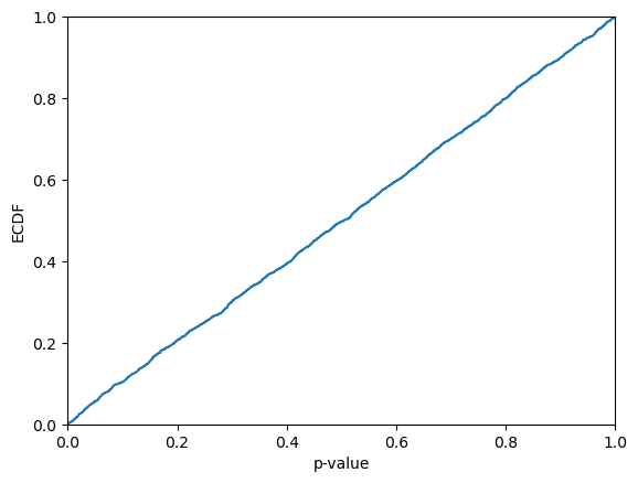
KS-test: 0.1201641198156913
Normalized conformal regressors#
The above intervals are not normalized, i.e., they are all of the same size (at least before they are cut). We could make the intervals more informative through normalization using difficulty estimates; more difficult instances will be assigned wider intervals. We can use a DifficultyEstimator, as imported from crepes.extras, for this purpose. It can be used to estimate the difficulty by using k-nearest neighbors in three different ways: i) by the (Euclidean) distances to the nearest
neighbors, ii) by the standard deviation of the targets of the nearest neighbors, and iii) by the absolute errors of the k nearest neighbors.
A small value (beta) is added to the estimates, which may be given through a (named) argument to the fit method; we will just use the default for this, i.e., beta=0.01. In order to make the beta value have the same effect across different estimators, we may opt for normalizing the difficulty estimates (using min-max scaling) by setting scaler=True. It should be noted that this comes with a computational cost; for estimators based on the k-nearest neighbor, a leave-one-out protocol is
employed to find the minimum and maximum distances that are used by the scaler.
We will first consider just using the first option (distances to the k-nearest neighbors) to produce normalized conformal regressors, using the default number of nearest neighbors, i.e., k=25.
[59]:
de_knn = DifficultyEstimator()

de_knn.fit(X=X_prop_train, scaler=True)

display(de_knn)

sigmas_cal_knn_dist = de_knn.apply(X_cal)

cr_norm_knn_dist = ConformalRegressor()

cr_norm_knn_dist.fit(residuals_cal, sigmas=sigmas_cal_knn_dist)

display(cr_norm_knn_dist)
DifficultyEstimator(fitted=True, type=knn, k=25, target=none, scaler=True, beta=0.01, oob=False)
ConformalRegressor(fitted=True, normalized=True, mondrian=False)
To generate prediction intervals for the test set, we need difficulty estimates for the latter too, which we get in the same way as for the calibration objects.
[60]:
sigmas_test_knn_dist = de_knn.apply(X_test)

intervals_norm_knn_dist = cr_norm_knn_dist.predict_int(y_hat_test,
                                                       sigmas=sigmas_test_knn_dist,
                                                       y_min=0, y_max=1)

display(intervals_norm_knn_dist)
array([[0.03628799, 0.06038621],
       [0.05363784, 0.13281694],
       [0.06890303, 0.08245828],
       ...,
       [0.02678008, 0.06357846],
       [0.03045481, 0.06381656],
       [0.00722417, 0.04810029]])
Alternatively, we could estimate the difficulty using the standard deviation of the targets of the nearest neighbors; we specify this by providing the targets too:
[61]:
de_knn_std = DifficultyEstimator()

de_knn_std.fit(X=X_prop_train, y=y_prop_train, scaler=True)

display(de_knn_std)

sigmas_cal_knn_std = de_knn_std.apply(X_cal)

cr_norm_knn_std = ConformalRegressor()

cr_norm_knn_std.fit(residuals_cal, sigmas=sigmas_cal_knn_std)

display(cr_norm_knn_std)
DifficultyEstimator(fitted=True, type=knn, k=25, target=labels, scaler=True, beta=0.01, oob=False)
ConformalRegressor(fitted=True, normalized=True, mondrian=False)
… and similarly for the test objects:
[62]:
sigmas_test_knn_std = de_knn_std.apply(X_test)

intervals_norm_knn_std = cr_norm_knn_std.predict_int(y_hat_test,
                                                     sigmas=sigmas_test_knn_std,
                                                     y_min=0, y_max=1)

display(intervals_norm_knn_std)
array([[0.0359405 , 0.0607337 ],
       [0.04231828, 0.1441365 ],
       [0.05340549, 0.09795582],
       ...,
       [0.02701465, 0.0633439 ],
       [0.0313224 , 0.06294897],
       [0.01948303, 0.03584143]])
A third option is to use (absolute) residuals for the reference objects. For a model that overfits the training data, it can be a good idea to use a separate set of (reference) objects and labels from which the residuals could be calculated, rather than using the original training data. Since we in this case have trained a random forest, we opt for estimating the residuals by using the out-of-bag predictions for the training instances. (This was made possible by setting oob_score=True for
the RandomForestRegressor above.)
To inform the fit method that this is what we want to do, we provide a value for residuals, instead of y as we did above for the option to use the (standard deviation of) the targets.
[63]:
oob_predictions = learner_prop.oob_prediction_

residuals_oob = y_prop_train - oob_predictions

de_knn_res = DifficultyEstimator()

de_knn_res.fit(X=X_prop_train, residuals=residuals_oob, scaler=True)

display(de_knn_res)

sigmas_cal_knn_res = de_knn_res.apply(X_cal)

cr_norm_knn_res = ConformalRegressor()

cr_norm_knn_res.fit(residuals_cal, sigmas=sigmas_cal_knn_res)

display(cr_norm_knn_res)
DifficultyEstimator(fitted=True, type=knn, k=25, target=residuals, scaler=True, beta=0.01, oob=False)
ConformalRegressor(fitted=True, normalized=True, mondrian=False)
… and again, the difficulty estimates are formed in the same way for the test objects:
[64]:
sigmas_test_knn_res = de_knn_res.apply(X_test)

intervals_norm_knn_res = cr_norm_knn_res.predict_int(y_hat_test,
                                                     sigmas=sigmas_test_knn_res,
                                                     y_min=0, y_max=1)

display(intervals_norm_knn_res)
array([[0.02140072, 0.07527348],
       [0.04364874, 0.14280604],
       [0.04936139, 0.10199992],
       ...,
       [0.02505443, 0.06530412],
       [0.0272979 , 0.06697347],
       [0.01561361, 0.03971085]])
In case we have trained an ensemble model, like a RandomForestRegressor, we could alternatively request DifficultyEstimator to estimate the difficulty by the variance of the predictions of the constituent models. This requires us to provide the trained model learner as input to fit, assuming that learner.estimators_ is a collection of base models, each implementing the predict method; this holds e.g., for RandomForestRegressor. A set of objects (X) has to be
provided only if we employ scaling (scaler=True).
[65]:
de_var = DifficultyEstimator()

de_var.fit(X=X_prop_train, learner=learner_prop, scaler=True)

display(de_var)

sigmas_cal_var = de_var.apply(X_cal)

cr_norm_var = ConformalRegressor()

cr_norm_var.fit(residuals_cal, sigmas=sigmas_cal_var)

display(cr_norm_var)
DifficultyEstimator(fitted=True, type=variance, scaler=True, beta=0.01, oob=False)
ConformalRegressor(fitted=True, normalized=True, mondrian=False)
The difficulty estimates for the test set are generated in the same way:
[66]:
sigmas_test_var = de_var.apply(X_test)

intervals_norm_var = cr_norm_var.predict_int(y_hat_test,
                                             sigmas=sigmas_test_var,
                                             y_min=0, y_max=1)

display(intervals_norm_var)
array([[0.03132678, 0.06534742],
       [0.06915468, 0.11730011],
       [0.05670411, 0.0946572 ],
       ...,
       [0.02916435, 0.0611942 ],
       [0.03100515, 0.06326622],
       [0.01105415, 0.04427031]])
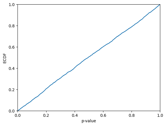
We can use predict_p to get the p-values also for normalized conformal regressors:
[67]:
p_values = cr_norm_var.predict_p(y_hat_test, y_test, sigmas=sigmas_test_var)

display(p_values)

plt.ecdf(p_values)
plt.xlim(0,1)
plt.xlabel("p-value")
plt.ylabel("ECDF")
plt.show()

print(f"KS-test: {kstest(p_values, "uniform").pvalue}")
array([0.60291613, 0.30023093, 0.28093901, ..., 0.15361843, 0.92208377,
       0.93213808])

KS-test: 0.10455479605928064
Mondrian conformal regressors#
An alternative way of generating prediction intervals of varying size is to divide the object space into non-overlapping so-called Mondrian categories. A Mondrian conformal regressor is formed by providing the names of the categories as an additional argument, named bins, for the fit method.
Here we employ the helper function binning, imported from crepes.extras, which given a list/array of values returns an array of the same length with the assigned bins. If the optional argument bins is an integer, the function will divide the values into equal-sized bins and return both the assigned bins and the bin boundaries. If bins instead is a set of bin boundaries, the function will just return the assigned bins.
We can form the Mondrian categories in any way we like, as long as we only use information that is available for both calibration and test instances; this means that we may not use the target values for this purpose, since these will typically not be available for the test instances. We will form categories by binning of the difficulty estimates, here using the ones previously produced using the standard deviations of the nearest neighbor targets.
[68]:
bins_cal, bin_thresholds = binning(sigmas_cal_var, bins=20)

cr_mond = ConformalRegressor()

cr_mond.fit(residuals_cal, bins=bins_cal)

display(cr_mond)
ConformalRegressor(fitted=True, normalized=False, mondrian=True)
Let us now obtain the categories for the test instances using the same Mondrian categorization, i.e., bin borders.
[69]:
bins_test = binning(sigmas_test_var, bins=bin_thresholds)
… and now we can form prediction intervals for the test instances.
[70]:
intervals_mond = cr_mond.predict_int(y_hat_test, bins=bins_test, y_min=0, y_max=1)

display(intervals_mond)
array([[0.03338259, 0.06329161],
       [0.05830384, 0.12815095],
       [0.05459185, 0.09676946],
       ...,
       [0.03242485, 0.0579337 ],
       [0.03438126, 0.05989011],
       [0.00968845, 0.04563602]])
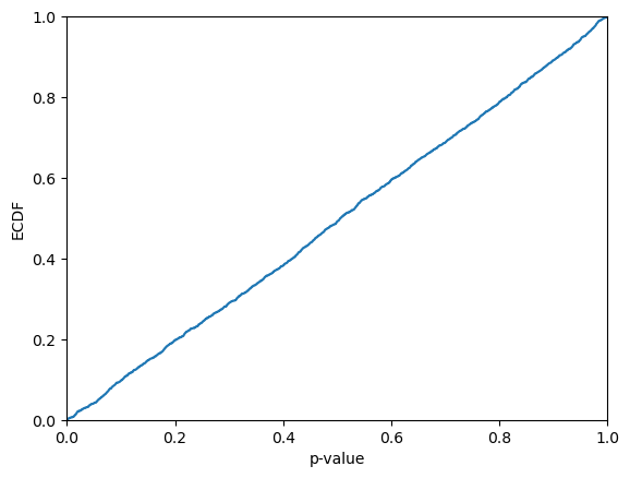
We can use predict_p to get the p-values also for Mondrian conformal regressors:
[71]:
p_values = cr_mond.predict_p(y_hat_test, y_test, bins=bins_test)

display(p_values)

plt.ecdf(p_values)
plt.xlim(0,1)
plt.xlabel("p-value")
plt.ylabel("ECDF")
plt.show()

print(f"KS-test: {kstest(p_values, "uniform").pvalue}")
array([0.57832057, 0.43596155, 0.38506015, ..., 0.08140979, 0.92507083,
       0.95499249])
KS-test: 0.03513808210229763
Investigating the prediction intervals#
Let us first put all the intervals in a dictionary.
[72]:
prediction_intervals = {
    "Std CR":intervals_std,
    "Norm CR knn dist":intervals_norm_knn_dist,
    "Norm CR knn std":intervals_norm_knn_std,
    "Norm CR knn res":intervals_norm_knn_res,
    "Norm CR var":intervals_norm_var,
    "Mond CR":intervals_mond,
}
Let us see what fraction of the intervals that contain the true targets and how large the intervals are.
[73]:
coverages = []
mean_sizes = []
median_sizes = []

for name in prediction_intervals.keys():
    intervals = prediction_intervals[name]
    coverages.append(np.sum([1 if (y_test[i]>=intervals[i,0] and
                                   y_test[i]<=intervals[i,1]) else 0
                            for i in range(len(y_test))])/len(y_test))
    mean_sizes.append((intervals[:,1]-intervals[:,0]).mean())
    median_sizes.append(np.median((intervals[:,1]-intervals[:,0])))

pred_int_df = pd.DataFrame({"Coverage":coverages,
                            "Mean size":mean_sizes,
                            "Median size":median_sizes},
                           index=list(prediction_intervals.keys()))

pred_int_df.loc["Mean"] = [pred_int_df["Coverage"].mean(),
                           pred_int_df["Mean size"].mean(),
                           pred_int_df["Median size"].mean()]

display(pred_int_df.round(4))
| Coverage | Mean size | Median size | |
|---|---|---|---|
| Std CR | 0.9434 | 0.0589 | 0.0603 |
| Norm CR knn dist | 0.9447 | 0.0570 | 0.0466 |
| Norm CR knn std | 0.9456 | 0.0592 | 0.0467 |
| Norm CR knn res | 0.9558 | 0.0583 | 0.0463 |
| Norm CR var | 0.9477 | 0.0507 | 0.0358 |
| Mond CR | 0.9572 | 0.0549 | 0.0412 |
| Mean | 0.9491 | 0.0565 | 0.0461 |
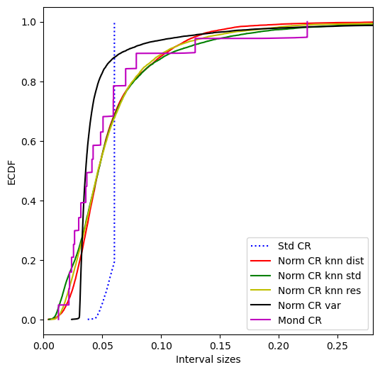
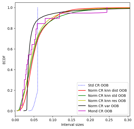
Let us look at the distribution of the interval sizes.
[74]:
interval_sizes = {}
for name in prediction_intervals.keys():
    interval_sizes[name] = prediction_intervals[name][:,1] \
    - prediction_intervals[name][:,0]

plt.figure(figsize=(6,6))
plt.ylabel("ECDF")
plt.xlabel("Interval sizes")
plt.xlim(0,interval_sizes["Mond CR"].max()*1.25)

colors = ["b","r","g","y","k","m","c","orange"]

for i, name in enumerate(interval_sizes.keys()):
    if "Std" in name:
        style = "dotted"
    else:
        style = "solid"
    plt.plot(np.sort(interval_sizes[name]),
             [i/len(interval_sizes[name])
              for i in range(1,len(interval_sizes[name])+1)],
             linestyle=style, c=colors[i], label=name)

plt.legend()
plt.show()
Evaluating the conformal regressors#
Let us put the six above conformal regressors in a dictionary, together with the corresponding difficulty estimates for the test instances (if any).
[75]:
all_cr = {
    "Std CR": (cr_std, []),
    "Norm CR knn dist": (cr_norm_knn_dist, sigmas_test_knn_dist),
    "Norm CR knn std": (cr_norm_knn_std, sigmas_test_knn_std),
    "Norm CR knn res": (cr_norm_knn_res, sigmas_test_knn_res),
    "Norm CR var" : (cr_norm_var, sigmas_test_var),
    "Mond CR": (cr_mond, sigmas_test_var),
}
Let us evaluate them using three confidence levels on the test set. We could specify a subset of the metrics to use by the named metrics argument of the evaluate method; here we use all, which is the default.
Note that the arguments sigmas and bins can always be provided, but they will be ignored by conformal regressors not using them, e.g., both arguments will be ignored by the standard conformal regressors.
[76]:
confidence_levels = [0.9,0.95,0.99]

names = list(all_cr.keys())

all_results = {}

for confidence in confidence_levels:
    for name in names:
        all_results[(name,confidence)] = all_cr[name][0].evaluate(
        y_hat_test, y_test, sigmas=all_cr[name][1],
        bins=bins_test, confidence=confidence,
        y_min=0, y_max=1)

results_df = pd.DataFrame(columns=pd.MultiIndex.from_product(
    [names,confidence_levels]), index=list(list(
    all_results.values())[0].keys()))

for key in all_results.keys():
    results_df[key] = all_results[key].values()

display(results_df.round(4))
| Std CR | Norm CR knn dist | Norm CR knn std | Norm CR knn res | Norm CR var | Mond CR | |||||||||||||
|---|---|---|---|---|---|---|---|---|---|---|---|---|---|---|---|---|---|---|
| 0.90 | 0.95 | 0.99 | 0.90 | 0.95 | 0.99 | 0.90 | 0.95 | 0.99 | 0.90 | 0.95 | 0.99 | 0.90 | 0.95 | 0.99 | 0.90 | 0.95 | 0.99 | |
| error | 0.1032 | 0.0566 | 0.0100 | 0.1108 | 0.0553 | 0.0075 | 0.1013 | 0.0544 | 0.0082 | 0.0978 | 0.0442 | 0.0081 | 0.1023 | 0.0523 | 0.0106 | 0.0908 | 0.0428 | 0.0060 |
| eff_mean | 0.0415 | 0.0589 | 0.1267 | 0.0431 | 0.0570 | 0.1013 | 0.0459 | 0.0592 | 0.1025 | 0.0424 | 0.0583 | 0.0954 | 0.0405 | 0.0507 | 0.0789 | 0.0433 | 0.0549 | 0.1080 |
| eff_med | 0.0417 | 0.0603 | 0.1266 | 0.0352 | 0.0466 | 0.0836 | 0.0361 | 0.0467 | 0.0825 | 0.0336 | 0.0463 | 0.0769 | 0.0284 | 0.0358 | 0.0575 | 0.0299 | 0.0412 | 0.0746 |
| ks_test | 0.1218 | 0.1145 | 0.1183 | 0.0051 | 0.0052 | 0.0049 | 0.0213 | 0.0226 | 0.0219 | 0.0208 | 0.0205 | 0.0206 | 0.1074 | 0.1041 | 0.1118 | 0.0422 | 0.0338 | 0.0288 |
| time_fit | 0.0001 | 0.0001 | 0.0001 | 0.0001 | 0.0001 | 0.0001 | 0.0000 | 0.0000 | 0.0000 | 0.0001 | 0.0001 | 0.0001 | 0.0000 | 0.0000 | 0.0000 | 0.0003 | 0.0003 | 0.0003 |
| time_evaluate | 0.1568 | 0.1293 | 0.1340 | 0.1404 | 0.1456 | 0.1378 | 0.1396 | 0.1360 | 0.1378 | 0.1450 | 0.1421 | 0.1383 | 0.1338 | 0.1299 | 0.1291 | 0.0874 | 0.0870 | 0.0895 |
Semi-online conformal regressors#
Similar to semi-online conformal classifiers, we may consider employing online calibration also for conformal regressors, i.e., continuously updating the calibration set after making each prediction. This is achieved by the methods predict_int_online and predict_p_online, and also (optionally) through the evaluate method.
Online calibration with a fitted conformal regressor#
Here we will compute p-values for the correct targets in an online fashion for some of the above fitted conformal regressors. Let us start with the standard (non-normalized) conformal regressor.
[77]:
p_values = cr_std.predict_p_online(y_hat_test, y_test)

display(p_values)

plt.ecdf(p_values)
plt.xlim(0,1)
plt.xlabel("p-value")
plt.ylabel("ECDF")
plt.show()

print(f"KS-test: {kstest(p_values, "uniform").pvalue}")
array([0.63872613, 0.26222725, 0.3203761 , ..., 0.26466162, 0.93186175,
       0.94000615])

KS-test: 0.7173594333102566
For the normalized conformal regressor, the non-conformity scores for the test set also involves the difficulty estimates (sigmas).
[78]:
p_values = cr_norm_var.predict_p_online(y_hat_test, y_test,
                                        sigmas=sigmas_test_var)

display(p_values)

plt.ecdf(p_values)
plt.xlim(0,1)
plt.xlabel("p-value")
plt.ylabel("ECDF")
plt.show()

print(f"KS-test: {kstest(p_values, "uniform").pvalue}")
array([0.60281752, 0.30028096, 0.28091112, ..., 0.15521915, 0.92130623,
       0.93235606])

KS-test: 0.802763821409657
For the Mondrian conformal regressor, we need to provide the categories for the test objects:
[79]:
p_values = cr_mond.predict_p_online(y_hat_test, y_test, bins=bins_test)

display(p_values)

plt.ecdf(p_values)
plt.xlim(0,1)
plt.xlabel("p-value")
plt.ylabel("ECDF")
plt.show()

print(f"KS-test: {kstest(p_values, "uniform").pvalue}")
array([0.57568383, 0.43468862, 0.38252884, ..., 0.08580778, 0.91065373,
       0.92513067])

KS-test: 0.37455439825133596
Similarly, we can obtain prediction intervals using online calibration:
[80]:
cr_std.predict_int_online(y_hat_test, y_test, y_min=0, y_max=1, confidence=0.9)
[80]:
array([[0.02749642, 0.06917779],
       [0.07238671, 0.11406808],
       [0.05483997, 0.09652134],
       ...,
       [0.02390627, 0.06645227],
       [0.02586269, 0.06840868],
       [0.00638923, 0.04893523]])
[81]:
cr_norm_var.predict_int_online(y_hat_test, y_test, sigmas=sigmas_test_var,
                               y_min=0, y_max=1, confidence=0.9)
[81]:
array([[0.0348651 , 0.0618091 ],
       [0.07416205, 0.11229273],
       [0.06065142, 0.09070988],
       ...,
       [0.03238266, 0.05797589],
       [0.03424669, 0.06002467],
       [0.01439166, 0.0409328 ]])
[82]:
cr_mond.predict_int_online(y_hat_test, y_test, bins=bins_test,
                           y_min=0, y_max=1, confidence=0.9)
[82]:
array([[0.03723164, 0.05944256],
       [0.06736352, 0.11909126],
       [0.05875411, 0.09260719],
       ...,
       [0.03556025, 0.05479829],
       [0.03749516, 0.05677621],
       [0.01694978, 0.03837468]])
By default, the test objects and labels are sequentially added to the existing calibration set, i.e., the one used when fitting the conformal regressor. We may set the warm_start option to False, if we would like to ignore the original calibration set. Note that the initial predictions tend to be very (maximally) wide, before we have a sufficiently large calibration set to allow for providing tighter intervals at the specified level of confidence.
[83]:
cr_std.predict_int_online(y_hat_test, y_test, y_min=0, y_max=1, confidence=0.9,
                      warm_start=False)
[83]:
array([[0.        , 1.        ],
       [0.        , 1.        ],
       [0.        , 1.        ],
       ...,
       [0.02365745, 0.0667011 ],
       [0.02561386, 0.06865751],
       [0.00614041, 0.04918405]])
[84]:
cr_norm_var.predict_int_online(y_hat_test, y_test, sigmas=sigmas_test_var,
                               y_min=0, y_max=1, confidence=0.9, warm_start=False)
[84]:
array([[0.        , 1.        ],
       [0.        , 1.        ],
       [0.        , 1.        ],
       ...,
       [0.03232396, 0.05803459],
       [0.03418757, 0.0600838 ],
       [0.01433079, 0.04099368]])
[85]:
cr_mond.predict_int_online(y_hat_test, y_test, bins=bins_test, y_min=0, y_max=1,
                           confidence=0.9, warm_start=False)
[85]:
array([[0.        , 1.        ],
       [0.        , 1.        ],
       [0.        , 1.        ],
       ...,
       [0.03553875, 0.0548198 ],
       [0.03743321, 0.05683816],
       [0.01728243, 0.03804203]])
We may also evaluate the conformal regressors using online calibration, by specifying online=True for the evaluate method:
[86]:
cr_std.evaluate(y_hat_test, y_test, confidence=0.99, y_min=0, y_max=1,
                online=True)
[86]:
{'error': 0.00990099009900991,
 'eff_mean': 0.12679320340457326,
 'eff_med': 0.1266798523278687,
 'ks_test': 0.726536687128762,
 'time_fit': 0.00014257431030273438,
 'time_evaluate': 0.24435162544250488}
[87]:
cr_norm_var.evaluate(y_hat_test, y_test, sigmas=sigmas_test_var,
                     confidence=0.99, y_min=0, y_max=1, online=True)
[87]:
{'error': 0.009993522716757686,
 'eff_mean': 0.08062719441140523,
 'eff_med': 0.05894043489803322,
 'ks_test': 0.8097871839387928,
 'time_fit': 3.814697265625e-05,
 'time_evaluate': 0.24166560173034668}
[88]:
cr_mond.evaluate(y_hat_test, y_test, bins=bins_test, confidence=0.99,
                 y_min=0, y_max=1, online=True)
[88]:
{'error': 0.007680207273063733,
 'eff_mean': 0.09012272547890991,
 'eff_med': 0.06108359344262293,
 'ks_test': 0.372543807529204,
 'time_fit': 0.00033545494079589844,
 'time_evaluate': 0.13530421257019043}
Again, we may consider ignoring the original calibration set by setting warm_start=False:
[89]:
cr_std.evaluate(y_hat_test, y_test, confidence=0.99, y_min=0, y_max=1,
                online=True, warm_start=False)
[89]:
{'error': 0.009993522716757686,
 'eff_mean': 0.13562933886475312,
 'eff_med': 0.12745168708196725,
 'ks_test': 0.7276080599350894,
 'time_fit': 0.00014257431030273438,
 'time_evaluate': 0.24033451080322266}
[90]:
cr_norm_var.evaluate(y_hat_test, y_test, sigmas=sigmas_test_var, confidence=0.99,
                     y_min=0, y_max=1, online=True, warm_start=False)
[90]:
{'error': 0.009623392245766582,
 'eff_mean': 0.09002682657313098,
 'eff_med': 0.05985148998481839,
 'ks_test': 0.8076587518875717,
 'time_fit': 3.814697265625e-05,
 'time_evaluate': 0.24507617950439453}
[91]:
cr_mond.evaluate(y_hat_test, y_test, bins=bins_test, confidence=0.99,
                 y_min=0, y_max=1, online=True, warm_start=False)
[91]:
{'error': 0.00666234847783842,
 'eff_mean': 0.2549119092780767,
 'eff_med': 0.07982348065573774,
 'ks_test': 0.3467164438408936,
 'time_fit': 0.00033545494079589844,
 'time_evaluate': 0.1332721710205078}
Online calibration without an initial calibration set#
Since the calibration set is incrementally extended during online calibration, we may consider starting with an empty calibration set; this allows us to use the full training set when fitting the underlying model.
[92]:
rf_full = RandomForestRegressor(n_jobs=-1, n_estimators=500)

rf_full.fit(X_train, y_train)
[92]:
RandomForestRegressor(n_estimators=500, n_jobs=-1)In a Jupyter environment, please rerun this cell to show the HTML representation or trust the notebook.
On GitHub, the HTML representation is unable to render, please try loading this page with nbviewer.org.
Parameters
| n_estimators | 500 | |
| criterion | 'squared_error' | |
| max_depth | None | |
| min_samples_split | 2 | |
| min_samples_leaf | 1 | |
| min_weight_fraction_leaf | 0.0 | |
| max_features | 1.0 | |
| max_leaf_nodes | None | |
| min_impurity_decrease | 0.0 | |
| bootstrap | True | |
| oob_score | False | |
| n_jobs | -1 | |
| random_state | None | |
| verbose | 0 | |
| warm_start | False | |
| ccp_alpha | 0.0 | |
| max_samples | None | |
| monotonic_cst | None |
Let us compute non-conformity scores for the test set using the model trained on the full training set:
[93]:
y_hat_full = rf_full.predict(X_test)
We may now create a conformal regressor, but this time without fitting a calibration set:
[94]:
cr_full = ConformalRegressor()
We may now obtain prediction intervals while sequentially updating the calibration set:
[95]:
cr_full.predict_int_online(y_hat_full, y_test, confidence=0.9)
[95]:
array([[      -inf,        inf],
       [      -inf,        inf],
       [      -inf,        inf],
       ...,
       [0.02328386, 0.0654074 ],
       [0.02554558, 0.06766911],
       [0.00571826, 0.0478418 ]])
If we provide also difficulty estimates (sigmas), we will obtain a normalized conformal regressor:
[96]:
cr_full.predict_int_online(y_hat_full, y_test, sigmas=sigmas_test_var, confidence=0.9)
[96]:
array([[      -inf,        inf],
       [      -inf,        inf],
       [      -inf,        inf],
       ...,
       [0.03175906, 0.05693221],
       [0.03392991, 0.05928478],
       [0.01372728, 0.03983278]])
We get a Mondrian regressor by providing the categories for the test set, here by dividing the predictions into seven intervals:
[97]:
bin_thresholds = [0.0, 0.02, 0.04, 0.06, 0.08, 0.1, 0.5, 1.0]
bins_test = binning(rf_full.predict(X_test), bin_thresholds)

cr_full.predict_int_online(y_hat_full, y_test, bins=bins_test, confidence=0.9)
[97]:
array([[      -inf,        inf],
       [      -inf,        inf],
       [      -inf,        inf],
       ...,
       [0.02965031, 0.05904096],
       [0.03191202, 0.06130267],
       [0.01624316, 0.03731691]])
Let us investigate the coverage and prediction interval size for each category:
[98]:
intervals = cr_full.predict_int_online(y_hat_full, y_test,
                                       bins=bins_test, y_min=0, y_max=1,
                                       confidence=0.9)
number = []
coverage = []
size = []

for c in range(len(bin_thresholds)-1):
    selection = bins_test == c
    number.append(np.sum(selection))
    coverage.append(np.sum(
        (intervals[selection,0] <= y_test[selection])& \
        (y_test[selection] <= intervals[selection,1]))/np.sum(selection))
    size.append(np.sum(intervals[selection,1]-\
                       intervals[selection,0])/np.sum(selection))

df = pd.DataFrame({"Number":number, "Coverage":coverage, "Size":size})
df.round(4)
[98]:
| Number | Coverage | Size | |
|---|---|---|---|
| 0 | 582 | 0.9192 | 0.0369 |
| 1 | 3201 | 0.8938 | 0.0235 |
| 2 | 2844 | 0.9079 | 0.0341 |
| 3 | 1867 | 0.8977 | 0.0439 |
| 4 | 1030 | 0.8932 | 0.0602 |
| 5 | 1280 | 0.9047 | 0.1462 |
| 6 | 3 | 1.0000 | 1.0000 |
We can use predict_p_online to get the p-values:
[99]:
p_values = cr_full.predict_p_online(y_hat_test, y_test, bins=bins_test)

display(p_values)

plt.ecdf(p_values)
plt.xlim(0,1)
plt.xlabel("p-value")
plt.ylabel("ECDF")
plt.show()

print(f"KS-test: {kstest(p_values, "uniform").pvalue}")
array([0.83436449, 0.39602701, 0.08942709, ..., 0.20290948, 0.93091173,
       0.91362726])

KS-test: 0.4066213612391897
We may also evaluate the conformal regressor using online calibration, by specifying online=True for the evaluate method:
[100]:
cr_full.evaluate(y_hat_full, y_test, y_min=0, y_max=1, confidence=0.9,
                 online=True)
[100]:
{'error': 0.10308133617100024,
 'eff_mean': 0.04195815434884792,
 'eff_med': 0.04158010072131149,
 'ks_test': 0.4803441170974383,
 'time_fit': None,
 'time_evaluate': 0.2064502239227295}
For Mondrian conformal regression, we just have to provide the categories:
[101]:
cr_full.evaluate(y_hat_full, y_test, bins=bins_test, y_min=0, y_max=1,
                 confidence=0.9, online=True)
[101]:
{'error': 0.09919496622559454,
 'eff_mean': 0.04883691480471517,
 'eff_med': 0.03076030845901649,
 'ks_test': 0.7384833785182272,
 'time_fit': None,
 'time_evaluate': 0.15108180046081543}
Out-of-bag calibration#
For conformal regressors that employ learners that use bagging, like random forests, we may consider an alternative strategy to dividing the original training set into a proper training and calibration set; we may use the out-of-bag (OOB) predictions, which allow us to use the full training set for both model building and calibration. It should be noted that this strategy does not come with the theoretical validity guarantee of the above (inductive) conformal regressors, due to that calibration and test instances are not handled in exactly the same way. In practice, however, conformal regressors based on out-of-bag predictions rarely do not meet the coverage requirements.
Standard conformal regressors with out-of-bag calibration#
Let us first generate a model from the full training set and then get the residuals using the OOB predictions; we rely on that the learner has an attribute oob_prediction_, which e.g. is the case for a RandomForestRegressor if oob_score is set to True when created.
[102]:
learner_full = RandomForestRegressor(n_jobs=-1, n_estimators=500,
                                     oob_score=True)

learner_full.fit(X_train, y_train)
[102]:
RandomForestRegressor(n_estimators=500, n_jobs=-1, oob_score=True)In a Jupyter environment, please rerun this cell to show the HTML representation or trust the notebook.
On GitHub, the HTML representation is unable to render, please try loading this page with nbviewer.org.
Parameters
| n_estimators | 500 | |
| criterion | 'squared_error' | |
| max_depth | None | |
| min_samples_split | 2 | |
| min_samples_leaf | 1 | |
| min_weight_fraction_leaf | 0.0 | |
| max_features | 1.0 | |
| max_leaf_nodes | None | |
| min_impurity_decrease | 0.0 | |
| bootstrap | True | |
| oob_score | True | |
| n_jobs | -1 | |
| random_state | None | |
| verbose | 0 | |
| warm_start | False | |
| ccp_alpha | 0.0 | |
| max_samples | None | |
| monotonic_cst | None |
Now we can obtain the residuals.
[103]:
oob_predictions = learner_full.oob_prediction_

residuals_oob = y_train - oob_predictions
We may now obtain a standard conformal regressor from these OOB residuals
[104]:
cr_std_oob = ConformalRegressor()

cr_std_oob.fit(residuals_oob)
[104]:
ConformalRegressor(fitted=True, normalized=False, mondrian=False)
… and apply it using the point predictions of the full model.
[105]:
y_hat_full = learner_full.predict(X_test)

intervals_std_oob = cr_std_oob.predict_int(y_hat_full, y_min=0, y_max=1)

display(intervals_std_oob)
array([[0.01826923, 0.07817608],
       [0.06093816, 0.12084501],
       [0.04522973, 0.10513657],
       ...,
       [0.01427348, 0.07418032],
       [0.01664922, 0.07655607],
       [0.        , 0.05678302]])
Normalized conformal regressors with out-of-bag calibration#
We may also generate normalized conformal regressors from the OOB predictions. The DifficultyEstimator can be used also for this purpose; for the k-nearest neighbor approaches, the difficulty of each object in the training set will be computed using a leave-one-out procedure, while for the variance-based approach the out-of-bag predictions will be employed.
By setting oob=True, we inform the fit method that we may request difficulty estimates for the provided set of objects; these will be retrieved by not providing any objects when calling the apply method.
Let us start with the k-nearest neighbor approach using distances only.
[106]:
de_knn_dist_oob = DifficultyEstimator()

de_knn_dist_oob.fit(X=X_train, scaler=True, oob=True)

display(de_knn_dist_oob)

sigmas_knn_dist_oob = de_knn_dist_oob.apply()

cr_norm_knn_dist_oob = ConformalRegressor()

cr_norm_knn_dist_oob.fit(residuals_oob, sigmas=sigmas_knn_dist_oob)
DifficultyEstimator(fitted=True, type=knn, k=25, target=none, scaler=True, beta=0.01, oob=True)
[106]:
ConformalRegressor(fitted=True, normalized=True, mondrian=False)
In order to apply the normalized OOB regressors to the test set, we need to generate difficulty estimates for the latter too.
[107]:
sigmas_test_knn_dist_oob = de_knn_dist_oob.apply(X_test)

intervals_norm_knn_dist_oob = cr_norm_knn_dist_oob.predict_int(
    y_hat_full, sigmas=sigmas_test_knn_dist_oob, y_min=0, y_max=1)

display(intervals_norm_knn_dist_oob)
array([[0.03592868, 0.06051664],
       [0.05122919, 0.13055398],
       [0.06613747, 0.08422883],
       ...,
       [0.02535723, 0.06309657],
       [0.02991777, 0.06328752],
       [0.0054855 , 0.04817368]])
For completeness, we will illustrate the use of out-of-bag calibration for the remaining approaches too. For k-nearest neighbors with labels, we do the following:
[108]:
de_knn_std_oob = DifficultyEstimator()

de_knn_std_oob.fit(X=X_train, y=y_train, scaler=True, oob=True)

display(de_knn_std_oob)

sigmas_knn_std_oob = de_knn_std_oob.apply()

cr_norm_knn_std_oob = ConformalRegressor()

cr_norm_knn_std_oob.fit(residuals=residuals_oob, sigmas=sigmas_knn_std_oob)

sigmas_test_knn_std_oob = de_knn_std_oob.apply(X_test)

intervals_norm_knn_std_oob = cr_norm_knn_std_oob.predict_int(
    y_hat_full, sigmas=sigmas_test_knn_std_oob, y_min=0, y_max=1)

display(intervals_norm_knn_std_oob)
DifficultyEstimator(fitted=True, type=knn, k=25, target=labels, scaler=True, beta=0.01, oob=True)
array([[0.03312216, 0.06332315],
       [0.03953184, 0.14225134],
       [0.0557293 , 0.094637  ],
       ...,
       [0.02404561, 0.06440819],
       [0.025169  , 0.06803629],
       [0.01830547, 0.03535371]])
A third option is to use k-nearest neighbors with (OOB) residuals:
[109]:
de_knn_res_oob = DifficultyEstimator()

de_knn_res_oob.fit(X=X_train, residuals=residuals_oob, scaler=True, oob=True)

display(de_knn_res_oob)

sigmas_knn_res_oob = de_knn_res_oob.apply()

cr_norm_knn_res_oob = ConformalRegressor()

cr_norm_knn_res_oob.fit(residuals_oob, sigmas=sigmas_knn_res_oob)

sigmas_test_knn_res_oob = de_knn_res_oob.apply(X_test)

intervals_norm_knn_res_oob = cr_norm_knn_res_oob.predict_int(
    y_hat_full, sigmas=sigmas_test_knn_res_oob, y_min=0, y_max=1)

display(intervals_norm_knn_res_oob)
DifficultyEstimator(fitted=True, type=knn, k=25, target=residuals, scaler=True, beta=0.01, oob=True)
array([[0.02172258, 0.07472273],
       [0.04911706, 0.13266611],
       [0.05735487, 0.09301143],
       ...,
       [0.02590461, 0.06254919],
       [0.03182191, 0.06138337],
       [0.01703558, 0.03662361]])
A fourth and final option for the normalized conformal regressors is to use variance as a difficulty estimate. We then leave labels and residuals out, but provide an (ensemble) learner. In contrast to when oob=False, we are here required to provide the (full) training set, from which the variance of the out-of-bag predictions will be computed. When applied to the test set, the full ensemble model will not be used to obtain the difficulty estimates, but instead a subset of the constituent
models is used, following what could be seen as post hoc assignment of each test instance to a bag.
[110]:
de_var_oob = DifficultyEstimator()

de_var_oob.fit(X=X_train, learner=learner_full, scaler=True, oob=True)

display(de_var_oob)

sigmas_var_oob = de_var_oob.apply()

cr_norm_var_oob = ConformalRegressor()

cr_norm_var_oob.fit(residuals_oob, sigmas=sigmas_var_oob)

sigmas_test_var_oob = de_var_oob.apply(X_test)

intervals_norm_var_oob = cr_norm_var_oob.predict_int(y_hat_full,
                                                     sigmas=sigmas_test_var_oob,
                                                     y_min=0, y_max=1)

display(intervals_norm_var_oob)
DifficultyEstimator(fitted=True, type=variance, scaler=True, beta=0.01, oob=True)
array([[0.03150298, 0.06494233],
       [0.06592113, 0.11586204],
       [0.0558818 , 0.0944845 ],
       ...,
       [0.02778142, 0.06067238],
       [0.02960762, 0.06359767],
       [0.00991146, 0.04374773]])
Mondrian conformal regressors with out-of-bag calibration#
We may form the categories using the difficulty estimates obtained from the OOB predictions. We here consider the difficulty estimates produced by the fourth above option (using variance) only.
[111]:
bins_oob, bin_thresholds_oob = binning(sigmas_var_oob, bins=20)

cr_mond_oob = ConformalRegressor()

cr_mond_oob.fit(residuals=residuals_oob, bins=bins_oob)
[111]:
ConformalRegressor(fitted=True, normalized=False, mondrian=True)
… and assign the categories for the test instances, …
[112]:
bins_test_oob = binning(sigmas_test_var_oob, bins=bin_thresholds_oob)
… and finally generate the prediction intervals.
[113]:
intervals_mond_oob = cr_mond_oob.predict_int(y_hat_full,
                                         bins=bins_test_oob,
                                         y_min=0, y_max=1)

display(intervals_mond_oob)
array([[0.0343643 , 0.06208102],
       [0.06155682, 0.12022635],
       [0.05284432, 0.09752198],
       ...,
       [0.03193711, 0.05651669],
       [0.0319638 , 0.06124149],
       [0.01297123, 0.04068795]])
Investigating the OOB prediction intervals#
[114]:
prediction_intervals = {
    "Std CR OOB":intervals_std_oob,
    "Norm CR knn dist OOB":intervals_norm_knn_dist_oob,
    "Norm CR knn std OOB":intervals_norm_knn_std_oob,
    "Norm CR knn res OOB":intervals_norm_knn_res_oob,
    "Norm CR var OOB":intervals_norm_var_oob,
    "Mond CR OOB":intervals_mond_oob,
}
Let us see what fraction of the intervals that contain the true targets and how large the intervals are.
[115]:
coverages = []
mean_sizes = []
median_sizes = []

for name in prediction_intervals.keys():
    intervals = prediction_intervals[name]
    coverages.append(np.sum([1 if (y_test[i]>=intervals[i,0] and
                                   y_test[i]<=intervals[i,1]) else 0
                            for i in range(len(y_test))])/len(y_test))
    mean_sizes.append((intervals[:,1]-intervals[:,0]).mean())
    median_sizes.append(np.median((intervals[:,1]-intervals[:,0])))

pred_int_df = pd.DataFrame({"Coverage":coverages,
                            "Mean size":mean_sizes,
                            "Median size":median_sizes},
                           index=list(prediction_intervals.keys()))

pred_int_df.loc["Mean"] = [pred_int_df["Coverage"].mean(),
                           pred_int_df["Mean size"].mean(),
                           pred_int_df["Median size"].mean()]

display(pred_int_df.round(4))
| Coverage | Mean size | Median size | |
|---|---|---|---|
| Std CR OOB | 0.9459 | 0.0585 | 0.0599 |
| Norm CR knn dist OOB | 0.9497 | 0.0569 | 0.0471 |
| Norm CR knn std OOB | 0.9472 | 0.0574 | 0.0448 |
| Norm CR knn res OOB | 0.9492 | 0.0539 | 0.0422 |
| Norm CR var OOB | 0.9483 | 0.0504 | 0.0359 |
| Mond CR OOB | 0.9504 | 0.0522 | 0.0349 |
| Mean | 0.9484 | 0.0549 | 0.0441 |
Let us look at the distribution of the interval sizes.
[116]:
interval_sizes = {}
for name in prediction_intervals.keys():
    interval_sizes[name] = prediction_intervals[name][:,1] \
    - prediction_intervals[name][:,0]

plt.figure(figsize=(6,6))
plt.ylabel("ECDF")
plt.xlabel("Interval sizes")
plt.xlim(0,interval_sizes["Mond CR OOB"].max()*1.25)

colors = ["b","r","g","y","k","m","c","orange"]

for i, name in enumerate(interval_sizes.keys()):
    if "Std" in name:
        style = "dotted"
    else:
        style = "solid"
    plt.plot(np.sort(interval_sizes[name]),
             [i/len(interval_sizes[name])
              for i in range(1,len(interval_sizes[name])+1)],
             linestyle=style, c=colors[i], label=name)

plt.legend()
plt.show()
Conformal Predictive Systems (CPS)#
Creating and fitting CPS#
Let us create and fit standard and normalized conformal predictive systems, using the residuals from the calibration set (as obtained in the previous section), as well two conformal predictive systems using out-of-bag residuals; with and without normalization. As can be seen, the input for fitting conformal predictive systems is on the same format as for the conformal regressors.
[117]:
cps_std = ConformalPredictiveSystem().fit(residuals_cal)

cps_norm = ConformalPredictiveSystem().fit(residuals_cal,
                                           sigmas=sigmas_cal_var)

cps_std_oob = ConformalPredictiveSystem().fit(residuals_oob)

cps_norm_oob = ConformalPredictiveSystem().fit(residuals_oob,
                                               sigmas=sigmas_var_oob)
Let us also create some Mondrian CPS, but in contrast to the Mondrian conformal regressors above, we here form the categories through binning of the predictions rather than binning of the difficulty estimates. We may use the latter, i.e., the sigmas, to obtain a normalized CPS for each category (bin).
[118]:
bins_cal, bin_thresholds = binning(y_hat_cal, bins=5)

cps_mond_std = ConformalPredictiveSystem().fit(residuals_cal,
                                               bins=bins_cal)

cps_mond_norm = ConformalPredictiveSystem().fit(residuals_cal,
                                                sigmas=sigmas_cal_var,
                                                bins=bins_cal)


bins_oob, bin_thresholds_oob = binning(oob_predictions, bins=5)

cps_mond_std_oob = ConformalPredictiveSystem().fit(residuals_oob,
                                                   bins=bins_oob)

cps_mond_norm_oob = ConformalPredictiveSystem().fit(residuals_oob,
                                                    sigmas=sigmas_var_oob,
                                                    bins=bins_oob)
Making predictions#
For the normalized approaches, we already have the difficulty estimates which are needed for the test instances. For the Mondrian approaches, we also need to assign the new categories to the test instances.
[119]:
bins_test = binning(y_hat_test, bins=bin_thresholds)

bins_test_oob = binning(y_hat_full, bins=bin_thresholds_oob)
The predict_p and predict_int methods work as for conformal regressors, i.e., to get p-values and prediction intervals. There are also some methods that are specific to conformal predictive systems; predict_percentiles and predict_cpds that are used for obtaining percentiles and conformal predictive distributions, respectively. In addition, we may employ the predict method, for which the output will depend on how we specify the input and which can be used for getting all of
the above by just one call.
Here we will obtain the p-values from cps_mond_norm for the true targets of the test set:
[120]:
p_values = cps_mond_norm.predict_p(y_hat_test, y_test, sigmas=sigmas_test_var,
                                   bins=bins_test, seed=123)

display(p_values)
array([0.74805262, 0.21639509, 0.1852622 , ..., 0.9340227 , 0.57518794,
       0.56124848])
Let us take a look at how the p-values are distributed. From the visual inspection they may appear be approximaly uniformly distributed; this is however not guaranteed, since the p-values are not independent (see further below for semi-online conformal predictive systems, for which this indeed holds). It is hence not very surprising if the Kolmogorov-Smirnov test allows us to reject that the p-values are sampled from a uniform distribution.
[121]:
plt.ecdf(p_values)
plt.xlim(0,1)
plt.xlabel("p-value")
plt.ylabel("ECDF")
plt.show()

print(f"KS-test: {kstest(p_values, "uniform").pvalue}")
KS-test: 0.0019516892048491992
We can get the same result through predict in the following way (since smoothing is enabled by default, we need to set the seed to get identical results):
[122]:
p_values = cps_mond_norm.predict(y_hat_test,
                                 sigmas=sigmas_test_var,
                                 bins=bins_test,
                                 y=y_test, seed=123)

display(p_values)
array([0.74805262, 0.21639509, 0.1852622 , ..., 0.9340227 , 0.57518794,
       0.56124848])
We can also request non-smoothed p-values, which are computed deterministically (a seed is hence not required to replicate the output):
[123]:
p_values = cps_mond_norm.predict_p(y_hat_test, y_test, sigmas_test_var,
                                   bins_test, smoothing=False)

display(p_values)
array([0.74861368, 0.21771218, 0.18669131, ..., 0.93530499, 0.5767098 ,
       0.56273063])
We can get the same result through predict in the following way:
[124]:
p_values = cps_mond_norm.predict(y_hat_test,
                                 sigmas=sigmas_test_var,
                                 bins=bins_test,
                                 y=y_test, smoothing=False)

display(p_values)
array([0.74861368, 0.21771218, 0.18669131, ..., 0.93530499, 0.5767098 ,
       0.56273063])
If we instead would like to get threshold values, such that the probability for the true target is less than the threshold for each test instance, we may request these through predict_percentiles or by providing lower_percentiles and/or upper_percentiles as input to the predict method. These denote (one or more) percentiles for which a lower (upper) value will be selected in case a percentile lies between two values (similar to interpolation="lower" and
interpolation="higher" in numpy.percentile).
Here we will obtain the lowest values from cps_mond_norm, such that the probability for the target values being less than these is at least 50%, first using predict_percentiles:
[125]:
thresholds = cps_mond_norm.predict_percentiles(y_hat_test, sigmas_test_var,
                                               bins_test, higher_percentiles=50)

display(thresholds)
array([0.04752931, 0.09246289, 0.07532108, ..., 0.04441875, 0.04636967,
       0.02746839])
Again, the same result can be obtained using the predict method:
[126]:
thresholds = cps_mond_norm.predict(y_hat_test, sigmas_test_var,
                                   bins_test, higher_percentiles=50)

display(thresholds)
array([0.04752931, 0.09246289, 0.07532108, ..., 0.04441875, 0.04636967,
       0.02746839])
We can also specify both target values and percentiles for the predict method; the resulting p-values will be returned in the first column, while any values corresponding to the lower percentiles will be included in the subsequent columns, followed by columns containing the values corresponding to the higher percentiles. The following call hence results in an array with five columns:
[127]:
results = cps_mond_norm.predict(y_hat_test,
                                sigmas=sigmas_test_var,
                                bins=bins_test,
                                y=y_test,
                                lower_percentiles=[2.5, 5],
                                higher_percentiles=[95, 97.5])

display(results)
array([[0.74747909, 0.03117374, 0.03354476, 0.06084538, 0.06601425],
       [0.21764835, 0.06842115, 0.07157618, 0.12037506, 0.12886095],
       [0.18549249, 0.05533979, 0.05840194, 0.09158912, 0.09629064],
       ...,
       [0.93494607, 0.02902026, 0.03125254, 0.0569556 , 0.061822  ],
       [0.57548715, 0.03086003, 0.03310842, 0.05899702, 0.06389855],
       [0.56201073, 0.01478018, 0.01631604, 0.03586697, 0.03975539]])
In addition to p-values and threshold values, we can request that the conformal predictive system returns the full conformal predictive distribution (CPD) for each test instance, as defined by the threshold values, either by the predict_cpds method or by setting return_cpds=True for the predict method . The format of the distributions vary with the type of conformal predictive system; for a standard and normalized CPS, the output is an array with a row for each test instance and a
column for each calibration instance (residual), while for a Mondrian CPS, the default output is a vector containing one CPD per test instance (since the number of values may vary between categories). If the desired output instead is an array of distributions per category, where all distributions in a category have the same number of columns, which in turn depends on the number of calibration instances in the corresponding category, then cpds_by_bins=True may be specified (for both methods).
In case return_cpds=True is specified together with y, lower_percentiles or higher_percentiles, the output of predict will be a pair, with the first element holding the results of the above type and the second element will contain the CPDs.
For the above Mondrian CPS, the following call to predict_cpds will result in a vector of distributions, with one element for each test instance.
[128]:
cpds = cps_mond_norm.predict_cpds(y_hat_test, sigmas_test_var, bins_test)

print(f"No. of test instances: {len(y_hat_test)}")
print(f"Shape of cpds: {cpds.shape}")
No. of test instances: 10807
Shape of cpds: (10807,)
The same result can be obtained with the following call to predict:
[129]:
cpds = cps_mond_norm.predict(y_hat_test,
                             sigmas=sigmas_test_var,
                             bins=bins_test,
                             return_cpds=True)

print(f"No. of test instances: {len(y_hat_test)}")
print(f"Shape of cpds: {cpds.shape}")
No. of test instances: 10807
Shape of cpds: (10807,)
If we instead would prefer to represent these distributions by one array per category, we set cpds_by_bins=True, noting that it will be a bit trickier to associate a test instance to a specific distribution.
[130]:
cpds = cps_mond_norm.predict_cpds(y_hat_test, sigmas_test_var, bins_test,
                                  cpds_by_bins=True)

for i, cpd in enumerate(cpds):
    print(f"bin {i}: {cpd.shape[0]} test instances, {cpd.shape[1]} threshold values")

print(f"No. of test instances: {sum([c.shape[0] for c in cpds])}")
bin 0: 2311 test instances, 541 threshold values
bin 1: 2035 test instances, 540 threshold values
bin 2: 2085 test instances, 540 threshold values
bin 3: 2097 test instances, 540 threshold values
bin 4: 2279 test instances, 541 threshold values
No. of test instances: 10807
The same result can be obtained with the following call to predict:
[131]:
cpds = cps_mond_norm.predict(y_hat_test,
                             sigmas=sigmas_test_var,
                             bins=bins_test,
                             return_cpds=True,
                             cpds_by_bins=True)

for i, cpd in enumerate(cpds):
    print(f"bin {i}: {cpd.shape[0]} test instances, {cpd.shape[1]} threshold values")

print(f"No. of test instances: {sum([c.shape[0] for c in cpds])}")
bin 0: 2311 test instances, 541 threshold values
bin 1: 2035 test instances, 540 threshold values
bin 2: 2085 test instances, 540 threshold values
bin 3: 2097 test instances, 540 threshold values
bin 4: 2279 test instances, 541 threshold values
No. of test instances: 10807
We may also plot the conformal predictive distribution for some test object. In case the calibration set is very large, you may consider plotting an approximation of the full distribution by using a grid of values for lower_percentiles or higher_percentiles, instead of setting return_cpds=True. For the Mondrian CPS, the size of the calibration set for each bin is reasonable in this case, so we may just use the distributions directly.
[132]:
cpds = cps_mond_norm_oob.predict(y_hat_full,
                                 bins=bins_test_oob,
                                 sigmas=sigmas_test_var_oob,
                                 return_cpds=True)

test_index = np.random.randint(len(y_hat_full)) # A test object is randomly selected
cpd = cpds[test_index]

p = np.array([i/len(cpd) for i in range(len(cpd))])

lower_index = np.where(p<=0.025)[0][-1]
mid_index = np.where(p>=0.50)[0][0]
upper_index = np.where(p>=0.975)[0][0]

low_percentile = cpd[lower_index]
median = cpd[mid_index]
high_percentile = cpd[upper_index]

plt.figure(figsize=(6,6))
plt.plot([y_hat_full[test_index],y_hat_full[test_index]],[0,1], color="tab:orange")
plt.plot([y_test[test_index],y_test[test_index]],[0,1], color="tab:red")
plt.xlabel("y")
plt.ylabel("Q(y)")
plt.ylim(0,1)

plt.plot([median,median],[0,1],"g--")
plt.plot([low_percentile,low_percentile],[0,1],"y--")
plt.legend(["ŷ","target","$y_{0.5}$","[$y_{0.025}$,$y_{0.975}$]"])
plt.plot([high_percentile,high_percentile],[0,1],"y--")
plt.plot(cpd,p, color="tab:blue")
rectangle = plt.Rectangle((low_percentile,0),
                          abs(high_percentile-low_percentile),1, color="y",
                          alpha=0.05)
plt.gca().add_patch(rectangle)
plt.show()
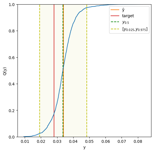
Investigating the coverage and size of extracted prediction intervals#
Let us investigate the extracted prediction intervals at the 95% confidence level. This is done by a specifying percentiles corresponding to the interval endpoints.
[133]:
all_cps = {"Std CPS":cps_std,
           "Std OOB CPS":cps_std_oob,
           "Norm CPS":cps_norm,
           "Norm OOB CPS":cps_norm_oob,
           "Mond CPS":cps_mond_std,
           "Mond OOB CPS":cps_mond_std_oob,
           "Mond norm CPS":cps_mond_norm,
           "Mond norm OOB CPS":cps_mond_norm_oob
          }

all_cps_intervals = {}

coverages = []
mean_sizes = []
median_sizes = []

for name in all_cps.keys():
    if "OOB" in name:
        intervals = all_cps[name].predict(y_hat_full,
                                          sigmas=sigmas_test_var_oob,
                                          bins=bins_test_oob,
                                          lower_percentiles=2.5,
                                          higher_percentiles=97.5,
                                          y_min=0, y_max=1)
    else:
        intervals = all_cps[name].predict(y_hat_test,
                                          sigmas=sigmas_test_var,
                                          bins=bins_test,
                                          lower_percentiles=2.5,
                                          higher_percentiles=97.5,
                                          y_min=0, y_max=1)
    all_cps_intervals[name] = intervals
    coverages.append(np.sum([1 if (y_test[i]>=intervals[i,0] and
                                   y_test[i]<=intervals[i,1]) else 0
                            for i in range(len(y_test))])/len(y_test))
    mean_sizes.append((intervals[:,1]-intervals[:,0]).mean())
    median_sizes.append(np.median((intervals[:,1]-intervals[:,0])))

pred_int_df = pd.DataFrame({"Coverage":coverages,
                            "Mean size":mean_sizes,
                            "Median size":median_sizes},
                           index=list(all_cps_intervals.keys()))

pred_int_df.loc["Mean"] = [pred_int_df["Coverage"].mean(),
                           pred_int_df["Mean size"].mean(),
                           pred_int_df["Median size"].mean()]

display(pred_int_df.round(4))
| Coverage | Mean size | Median size | |
|---|---|---|---|
| Std CPS | 0.9447 | 0.0600 | 0.0613 |
| Std OOB CPS | 0.9463 | 0.0600 | 0.0609 |
| Norm CPS | 0.9506 | 0.0522 | 0.0369 |
| Norm OOB CPS | 0.9511 | 0.0517 | 0.0367 |
| Mond CPS | 0.9523 | 0.0619 | 0.0406 |
| Mond OOB CPS | 0.9473 | 0.0574 | 0.0395 |
| Mond norm CPS | 0.9523 | 0.0548 | 0.0367 |
| Mond norm OOB CPS | 0.9488 | 0.0539 | 0.0350 |
| Mean | 0.9492 | 0.0565 | 0.0435 |
Investigating the distributions of extracted prediction intervals#
Let us take a look at the distribution of the interval sizes.
[134]:
cps_interval_sizes = {}

for name in all_cps_intervals.keys():
    cps_interval_sizes[name] = \
    all_cps_intervals[name][:,1] - all_cps_intervals[name][:,0]

plt.figure(figsize=(6,6))
plt.ylabel("ECDF")
plt.xlabel("Interval sizes")
plt.xlim(0,cps_interval_sizes["Mond OOB CPS"].max()*1.25)

colors = ["b","r","g","y","k","m", "gray", "orange"]

for i, name in enumerate(cps_interval_sizes.keys()):
    if "Std" in name:
        style = "dotted"
    else:
        style = "solid"
    plt.plot(np.sort(cps_interval_sizes[name]),
             [i/len(cps_interval_sizes[name])
              for i in range(1,len(cps_interval_sizes[name])+1)],
             linestyle=style, c=colors[i], label=name)

plt.legend()
plt.show()
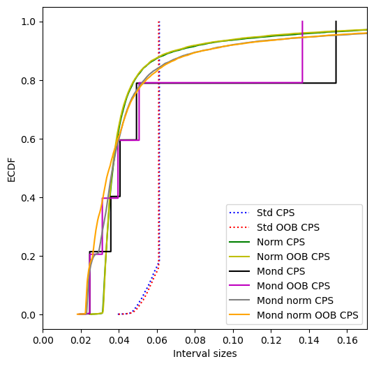
Extracting medians#
Let us take a look at the medians; they can be derived using either lower or higher interpolation, but ideally the differences should be small.
[135]:
all_cps_medians = {}

for name in all_cps.keys():
    if "OOB" in name:
        medians = all_cps[name].predict(y_hat_full,
                                        sigmas=sigmas_test_var_oob,
                                        bins=bins_test_oob,
                                        lower_percentiles=50,
                                        higher_percentiles=50)
    else:
        medians = all_cps[name].predict(y_hat_test,
                                        sigmas=sigmas_test_var,
                                        bins=bins_test,
                                        lower_percentiles=50,
                                        higher_percentiles=50)
    all_cps_medians[name] = medians
    print(name)
    print("\tMean difference of the medians:    {:.6f}".format((medians[:,1]-medians[:,0]).mean()))
    print("\tLargest difference of the medians: {:.6f}".format((medians[:,1]-medians[:,0]).max()))
Std CPS
        Mean difference of the medians:    0.000016
        Largest difference of the medians: 0.000016
Std OOB CPS
        Mean difference of the medians:    0.000005
        Largest difference of the medians: 0.000005
Norm CPS
        Mean difference of the medians:    0.000001
        Largest difference of the medians: 0.000083
Norm OOB CPS
        Mean difference of the medians:    0.000003
        Largest difference of the medians: 0.000175
Mond CPS
        Mean difference of the medians:    0.000040
        Largest difference of the medians: 0.000157
Mond OOB CPS
        Mean difference of the medians:    0.000001
        Largest difference of the medians: 0.000003
Mond norm CPS
        Mean difference of the medians:    0.000022
        Largest difference of the medians: 0.000262
Mond norm OOB CPS
        Mean difference of the medians:    0.000001
        Largest difference of the medians: 0.000006
Another view of the medians and prediction intervals#
[136]:
plt.subplots(len(all_cps_intervals.keys())//2,2,figsize=(12,24))

sorted_prop_indexes = np.argsort(y_hat_test)

sorted_full_indexes = np.argsort(y_hat_full)

alpha=0.2

for i, name in enumerate(all_cps_intervals.keys()):

    plt.subplot(len(all_cps_intervals.keys())//2,2,i+1)
    if "OOB" in name:
        indexes = sorted_full_indexes
        y_hat_ = y_hat_full
    else:
        indexes = sorted_prop_indexes
        y_hat_ = y_hat_test

    plt.title(name)
    plt.plot(y_hat_[indexes], all_cps_intervals[name][indexes,0],
             color="r", alpha=alpha)
    plt.plot(y_hat_[indexes], all_cps_intervals[name][indexes,1],
             color="r", alpha=alpha)
    plt.scatter(y_hat_[indexes],y_test[indexes],
                color="b", marker="o", alpha=alpha)
    plt.scatter(y_hat_[indexes],y_hat_[indexes],
                color="y", marker=".", alpha=alpha)
    plt.xlabel("predicted")
    plt.ylabel("endpoints")

plt.show()
Evaluating the CPS using a test set#
Let us evaluate the generated CPS using three confidence levels on the test set. We could specify a subset of the metrics to use by the metrics parameter of the evaluate method; here we use all metrics, which is the default
Note that values for the parameters sigmas and bins can always be provided, but they will be ignored by CPS that have not been fitted with such values, e.g., both arguments will be ignored by the standard CPS.
Note that CRPS takes some time to compute, in particular when the CPS have been fitted with larger calibration sets.
[137]:
confidence_levels = [0.9,0.95,0.99]

names = np.array(list(all_cps.keys()))

first_set = names[["OOB" not in name for name in names]]
second_set = names[["OOB" in name for name in names]]

for methods in [first_set, second_set]:
    all_cps_results = {}
    for confidence in confidence_levels:
        for name in methods:
            if "OOB" in name:
                all_cps_results[(name,confidence)] = all_cps[name].evaluate(
                    y_hat_full, y_test, sigmas=sigmas_test_var_oob,
                    bins=bins_test_oob, confidence=confidence,
                    y_min=0, y_max=1)
            else:
                all_cps_results[(name,confidence)] =  all_cps[name].evaluate(
                    y_hat_test, y_test, sigmas=sigmas_test_var,
                    bins=bins_test, confidence=confidence, y_min=0, y_max=1)

    cps_results_df = pd.DataFrame(columns=pd.MultiIndex.from_product(
        [methods,confidence_levels]), index=list(list(
        all_cps_results.values())[0].keys()))

    for key in all_cps_results.keys():
        cps_results_df[key] = all_cps_results[key].values()

    display(cps_results_df.round(4))
| Std CPS | Norm CPS | Mond CPS | Mond norm CPS | |||||||||
|---|---|---|---|---|---|---|---|---|---|---|---|---|
| 0.90 | 0.95 | 0.99 | 0.90 | 0.95 | 0.99 | 0.90 | 0.95 | 0.99 | 0.90 | 0.95 | 0.99 | |
| error | 0.1069 | 0.0553 | 0.0100 | 0.1033 | 0.0494 | 0.0070 | 0.1000 | 0.0477 | 0.0071 | 0.0982 | 0.0477 | 0.0061 |
| eff_mean | 0.0407 | 0.0600 | 0.1376 | 0.0403 | 0.0522 | 0.0887 | 0.0445 | 0.0619 | 0.1293 | 0.0437 | 0.0548 | 0.1037 |
| eff_med | 0.0409 | 0.0613 | 0.1407 | 0.0282 | 0.0369 | 0.0642 | 0.0305 | 0.0406 | 0.0798 | 0.0287 | 0.0367 | 0.0753 |
| time_fit | 0.0002 | 0.0002 | 0.0002 | 0.0002 | 0.0002 | 0.0002 | 0.0008 | 0.0008 | 0.0008 | 0.0004 | 0.0004 | 0.0004 |
| CRPS | 0.0077 | 0.0077 | 0.0077 | 0.0071 | 0.0071 | 0.0071 | 0.0074 | 0.0074 | 0.0074 | 0.0070 | 0.0070 | 0.0070 |
| ks_test | 0.0118 | 0.0123 | 0.0123 | 0.0003 | 0.0003 | 0.0003 | 0.0040 | 0.0049 | 0.0046 | 0.0019 | 0.0020 | 0.0022 |
| time_evaluate | 0.5627 | 0.5223 | 0.5094 | 0.5766 | 0.6103 | 0.6078 | 0.3441 | 0.3450 | 0.3388 | 0.3800 | 0.3908 | 0.3885 |
| Std OOB CPS | Norm OOB CPS | Mond OOB CPS | Mond norm OOB CPS | |||||||||
|---|---|---|---|---|---|---|---|---|---|---|---|---|
| 0.90 | 0.95 | 0.99 | 0.90 | 0.95 | 0.99 | 0.90 | 0.95 | 0.99 | 0.90 | 0.95 | 0.99 | |
| error | 0.1079 | 0.0537 | 0.0127 | 0.1041 | 0.0489 | 0.0092 | 0.1024 | 0.0527 | 0.0087 | 0.0992 | 0.0512 | 0.0074 |
| eff_mean | 0.0402 | 0.0600 | 0.1261 | 0.0392 | 0.0517 | 0.0802 | 0.0426 | 0.0574 | 0.1054 | 0.0422 | 0.0539 | 0.0871 |
| eff_med | 0.0404 | 0.0609 | 0.1333 | 0.0276 | 0.0367 | 0.0580 | 0.0293 | 0.0395 | 0.0669 | 0.0281 | 0.0350 | 0.0594 |
| time_fit | 0.0002 | 0.0002 | 0.0002 | 0.0001 | 0.0001 | 0.0001 | 0.0007 | 0.0007 | 0.0007 | 0.0010 | 0.0010 | 0.0010 |
| CRPS | 0.0076 | 0.0076 | 0.0076 | 0.0070 | 0.0070 | 0.0070 | 0.0073 | 0.0073 | 0.0073 | 0.0069 | 0.0069 | 0.0069 |
| ks_test | 0.1463 | 0.1452 | 0.1452 | 0.1050 | 0.1032 | 0.1033 | 0.0894 | 0.0864 | 0.0853 | 0.1340 | 0.1448 | 0.1469 |
| time_evaluate | 1.3020 | 1.1820 | 1.1895 | 1.3171 | 1.3376 | 1.2975 | 0.4622 | 0.4681 | 0.4574 | 0.5405 | 0.5335 | 0.5195 |
Semi-online conformal predictive systems#
Similar to semi-online conformal classifiers and regressors, we may consider employing online calibration also for conformal predictive systems, i.e., continuously updating the calibration set after making each prediction. This is achieved by the methods predict_p_online, predict_int_online, predict_percentiles_online and predict_cpds_online, and also (optionally) through the evaluate method.
Online calibration with a fitted conformal predictive system#
Here we will compute p-values for the correct targets in an online fashion for some of the above fitted conformal predictive systems. Let us start with the standard (non-normalized) conformal predictive system.
[138]:
p_values = cps_std.predict_p_online(y_hat_test, y_test)

display(p_values)

plt.ecdf(p_values)
plt.xlim(0,1)
plt.xlabel("p-value")
plt.ylabel("ECDF")
plt.show()

print(f"KS-test: {kstest(p_values, "uniform").pvalue}")
array([0.28358155, 0.85496346, 0.82321084, ..., 0.12369003, 0.43531529,
       0.43936203])

KS-test: 0.4980056130809166
For the normalized conformal predictive system, the non-conformity scores for the test set also involves the difficulty estimates (sigmas).
[139]:
p_values = cps_norm.predict_p_online(y_hat_test, y_test,
                                     sigmas=sigmas_test_var)

display(p_values)

plt.ecdf(p_values)
plt.xlim(0,1)
plt.xlabel("p-value")
plt.ylabel("ECDF")
plt.show()

print(f"KS-test: {kstest(p_values, "uniform").pvalue}")
array([0.26390876, 0.8335969 , 0.84585449, ..., 0.0783664 , 0.43066362,
       0.43608453])

KS-test: 0.28641385436207445
For the (non-normalized) Mondrian conformal predictive system, we need to provide the categories for the test objects:
[140]:
p_values = cps_mond_std.predict_p_online(y_hat_test, y_test,
                                         bins=bins_test)

display(p_values)

plt.ecdf(p_values)
plt.xlim(0,1)
plt.xlabel("p-value")
plt.ylabel("ECDF")
plt.show()

print(f"KS-test: {kstest(p_values, "uniform").pvalue}")
array([0.26097478, 0.6981751 , 0.77884335, ..., 0.0993303 , 0.42407576,
       0.44049014])

KS-test: 0.3135690377843878
For the normalized Mondrian conformal predictive system, we need to provide both difficulty estimates and Mondrian categories for the test objects:
[141]:
p_values = cps_mond_norm.predict_p_online(y_hat_test, y_test,
                                          sigmas=sigmas_test_var,
                                          bins=bins_test)

display(p_values)

plt.ecdf(p_values)
plt.xlim(0,1)
plt.xlabel("p-value")
plt.ylabel("ECDF")
plt.show()

print(f"KS-test: {kstest(p_values, "uniform").pvalue}")
array([0.25148752, 0.78235131, 0.81480265, ..., 0.07256446, 0.42037699,
       0.44126863])

KS-test: 0.2957658142517954
Similarly, we can obtain prediction intervals using online calibration:
[142]:
cps_std.predict_int_online(y_hat_test, y_test,
                           y_min=0, y_max=1, confidence=0.9)
[142]:
array([[0.02684778, 0.06777511],
       [0.07173807, 0.1126654 ],
       [0.05419133, 0.09511867],
       ...,
       [0.02468057, 0.0673269 ],
       [0.02663699, 0.06928331],
       [0.00716353, 0.04980986]])
[143]:
cps_norm.predict_int_online(y_hat_test, y_test,
                            sigmas=sigmas_test_var,
                            y_min=0, y_max=1, confidence=0.9)
[143]:
array([[0.0348583 , 0.06165476],
       [0.07415242, 0.11207431],
       [0.06064383, 0.0905377 ],
       ...,
       [0.03273422, 0.05847675],
       [0.03460079, 0.06052915],
       [0.01475624, 0.04145221]])
[144]:
cps_mond_std.predict_int_online(y_hat_test, y_test,
                                bins=bins_test,
                                y_min=0, y_max=1, confidence=0.9)
[144]:
array([[0.03213458, 0.06260149],
       [0.04830964, 0.15432365],
       [0.05464333, 0.09387855],
       ...,
       [0.03010165, 0.06055062],
       [0.03205806, 0.06250703],
       [0.01730779, 0.03621796]])
[145]:
cps_mond_norm.predict_int_online(y_hat_test, y_test,
                                 sigmas=sigmas_test_var, bins=bins_test,
                                 y_min=0, y_max=1, confidence=0.9)
[145]:
array([[0.03354476, 0.06084538],
[0.07157618, 0.12037506],
[0.05840194, 0.09158912],
...,
[0.03287984, 0.0578568 ],
[0.03474747, 0.05990473],
[0.01740657, 0.03626903]])
We can also get (lower and higher) percentiles using online calibration:
[146]:
cps_std.predict_percentiles_online(y_hat_test, y_test,
lower_percentiles = [2.5, 25],
higher_percentiles = [50, 75, 97.5],
y_min=0, y_max=1)
[146]:
array([[0.01906339, 0.04228044, 0.04774332, 0.05270552, 0.08033843],
[0.06395368, 0.08717254, 0.09263361, 0.09758698, 0.12522872],
[0.04640694, 0.06962399, 0.07508687, 0.08004024, 0.10768199],
...,
[0.01553511, 0.03925045, 0.04463477, 0.04971633, 0.07997685],
[0.01749152, 0.04120779, 0.04659118, 0.05167274, 0.08193326],
[0. , 0.02173433, 0.02711815, 0.03219929, 0.06245981]])
[147]:
cps_norm.predict_percentiles_online(y_hat_test, y_test,
sigmas=sigmas_test_var,
lower_percentiles = [2.5, 25],
higher_percentiles = [50, 75, 97.5],
y_min=0, y_max=1)
[147]:
array([[0.0317741 , 0.04311875, 0.04779595, 0.05217599, 0.06681162],
[0.06978771, 0.08585259, 0.09246157, 0.09865677, 0.1193722 ],
[0.05720313, 0.06985911, 0.07507695, 0.07996064, 0.09629064],
...,
[0.02992416, 0.04037905, 0.04472079, 0.04898536, 0.0633976 ],
[0.03177045, 0.04230209, 0.0466739 , 0.05096925, 0.06548552],
[0.01184211, 0.02268554, 0.02718801, 0.03160929, 0.04655532]])
[148]:
cps_mond_std.predict_percentiles_online(y_hat_test, y_test,
bins=bins_test,
lower_percentiles = [2.5, 25],
higher_percentiles = [50, 75, 97.5],
y_min=0, y_max=1)
[148]:
array([[0.02813117, 0.04249562, 0.04755792, 0.05197978, 0.068739 ],
[0.02873504, 0.0791388 , 0.09228393, 0.10463189, 0.18295758],
[0.0504721 , 0.06795771, 0.07532596, 0.08278247, 0.09974216],
...,
[0.0259794 , 0.03956782, 0.04445653, 0.04959634, 0.06626808],
[0.02793582, 0.04152423, 0.04642114, 0.05155806, 0.06822449],
[0.01510309, 0.02412928, 0.02756003, 0.03046197, 0.03943192]])
[149]:
cps_mond_norm.predict_percentiles_online(y_hat_test, y_test,
sigmas=sigmas_test_var,
bins=bins_test,
lower_percentiles = [2.5, 25],
higher_percentiles = [50, 75, 97.5],
y_min=0, y_max=1)
[149]:
array([[0.03117374, 0.04290548, 0.04752931, 0.05187139, 0.06601425],
[0.06842115, 0.08375286, 0.09246289, 0.1006292 , 0.12886095],
[0.05533979, 0.06870191, 0.07532108, 0.08197924, 0.09629064],
...,
[0.02959335, 0.04035159, 0.0445109 , 0.04911261, 0.06242445],
[0.03143725, 0.04227315, 0.04646488, 0.05112402, 0.06450535],
[0.01536541, 0.02404679, 0.02755122, 0.0305258 , 0.03933413]])
We can also obtain the full conformal predictive distributions (cpds) using online calibration. For standard and normalized conformal predictive systems, each cpd will contain one more value than the preceding, since the calibration set is growing by one element for each prediction.
[150]:
cpds = cps_norm.predict_cpds_online(y_hat_test, y_test, sigmas=sigmas_test_var)
plt.plot(np.arange(len(cpds)), [len(cpds[i]) for i in range(len(cpds))])
plt.xlabel("#test objects")
plt.ylabel("calibration set size")
plt.ylim(0)
plt.xlim(0)
plt.show()
For Mondrian conformal predictive systems, the calibration set for one of the categories will be extended with one element for each prediction; the size of the predicted cpd is dependent on which category the test object falls in.
[151]:
cpds = cps_mond_norm.predict_cpds_online(y_hat_test, y_test,
sigmas=sigmas_test_var,
bins=bins_test)
plt.plot(np.arange(len(cpds)), [len(cpds[i]) for i in range(len(cpds))])
plt.xlabel("#test objects")
plt.ylabel("calibration set size")
plt.ylim(0)
plt.xlim(0)
plt.show()
By default, the test objects and labels are sequentially added to the existing calibration set, i.e., the one used when fitting the conformal predictive system. We may set the warm_start option to False, if we would like to ignore the original calibration set. Note that the initial predictions tend to be very (maximally) wide, before we have a sufficiently large calibration set to allow for providing tighter intervals at the specified level of confidence.
[152]:
cps_std.predict_int_online(y_hat_test, y_test,
y_min=0, y_max=1, confidence=0.9,
warm_start=False)
[152]:
array([[0. , 1. ],
[0. , 1. ],
[0. , 1. ],
...,
[0.02503051, 0.06785296],
[0.02698692, 0.06980937],
[0.00751347, 0.05033591]])
[153]:
cps_norm.predict_int_online(y_hat_test, y_test,
sigmas=sigmas_test_var,
y_min=0, y_max=1, confidence=0.9,
warm_start=False)
[153]:
array([[0. , 1. ],
[0. , 1. ],
[0. , 1. ],
...,
[0.03284543, 0.05864411],
[0.03471281, 0.06069771],
[0.01487157, 0.04162577]])
[154]:
cps_mond_std.predict_int_online(y_hat_test, y_test,
bins=bins_test,
y_min=0, y_max=1, confidence=0.9,
warm_start=False)
[154]:
array([[0. , 1. ],
[0. , 1. ],
[0. , 1. ],
...,
[0.03020264, 0.06071408],
[0.03215905, 0.06267049],
[0.01760788, 0.03621925]])
[155]:
cps_mond_norm.predict_int_online(y_hat_test, y_test,
sigmas=sigmas_test_var, bins=bins_test,
y_min=0, y_max=1, confidence=0.9,
warm_start=False)
[155]:
array([[0. , 1. ],
[0. , 1. ],
[0. , 1. ],
...,
[0.03307603, 0.05798737],
[0.03494507, 0.06003624],
[0.01760497, 0.03636111]])
Similarly, we may disable warm_start also when requesting percentiles using online calibration:
[156]:
cps_std.predict_percentiles_online(y_hat_test, y_test,
lower_percentiles = [2.5, 25],
higher_percentiles = [50, 75, 97.5],
y_min=0, y_max=1,
warm_start=False)
[156]:
array([[0. , 0. , 1. , 1. , 1. ],
[0. , 0. , 0.09669357, 1. , 1. ],
[0. , 0. , 0.07914683, 1. , 1. ],
...,
[0.01535516, 0.03927687, 0.04464461, 0.0497556 , 0.08096355],
[0.01731157, 0.04123328, 0.04660102, 0.05171484, 0.08291996],
[0. , 0.02175983, 0.02712859, 0.03224138, 0.06344651]])
[157]:
cps_norm.predict_percentiles_online(y_hat_test, y_test,
sigmas=sigmas_test_var,
lower_percentiles = [2.5, 25],
higher_percentiles = [50, 75, 97.5],
y_min=0, y_max=1,
warm_start=False)
[157]:
array([[0. , 0. , 1. , 1. , 1. ],
[0. , 0. , 0.09813267, 1. , 1. ],
[0. , 0. , 0.07954749, 1. , 1. ],
...,
[0.03008621, 0.04041761, 0.04473057, 0.04903909, 0.06361055],
[0.03193367, 0.04233965, 0.04668374, 0.05102366, 0.06570001],
[0.01201016, 0.02272421, 0.02719836, 0.03166531, 0.04677616]])
[158]:
cps_mond_std.predict_percentiles_online(y_hat_test, y_test,
bins=bins_test,
lower_percentiles = [2.5, 25],
higher_percentiles = [50, 75, 97.5],
y_min=0, y_max=1,
warm_start=False)
[158]:
array([[0. , 0. , 1. , 1. , 1. ],
[0. , 0. , 1. , 1. , 1. ],
[0. , 0. , 1. , 1. , 1. ],
...,
[0.02600494, 0.03969374, 0.04450601, 0.04967186, 0.06660716],
[0.02796135, 0.04165015, 0.04646299, 0.05164797, 0.06856357],
[0.01504283, 0.02411449, 0.0275855 , 0.03055382, 0.03947872]])
[159]:
cps_mond_norm.predict_percentiles_online(y_hat_test, y_test,
sigmas=sigmas_test_var,
bins=bins_test,
lower_percentiles = [2.5, 25],
higher_percentiles = [50, 75, 97.5],
y_min=0, y_max=1,
warm_start=False)
[159]:
array([[0. , 0. , 1. , 1. , 1. ],
[0. , 0. , 1. , 1. , 1. ],
[0. , 0. , 1. , 1. , 1. ],
...,
[0.02986562, 0.04038556, 0.04456032, 0.04924359, 0.06271397],
[0.03171149, 0.04230737, 0.04651564, 0.05124249, 0.06479695],
[0.01537617, 0.02400839, 0.02758352, 0.03063811, 0.03943161]])
We may set the warm_start option to False also when obtaining the conformal predictive distributions; this means that the size of the cpds will equal the number of already seen test objects for standard and normalized conformal predictive systems.
[160]:
cpds = cps_std.predict_cpds_online(y_hat_test, y_test,
warm_start=False)
plt.plot(np.arange(len(cpds)), [len(cpds[i]) for i in range(len(cpds))])
plt.xlabel("#test objects")
plt.ylabel("calibration set size")
plt.ylim(0)
plt.xlim(0)
plt.show()
For Mondrian conformal predictive systems, the calibration set for each category will be initially empty when warm_start is disabled.
[161]:
cpds = cps_mond_std.predict_cpds_online(y_hat_test, y_test,
bins=bins_test,
warm_start=False)
plt.plot(np.arange(len(cpds)), [len(cpds[i]) for i in range(len(cpds))])
plt.xlabel("#test objects")
plt.ylabel("calibration set size")
plt.ylim(0)
plt.xlim(0)
plt.show()
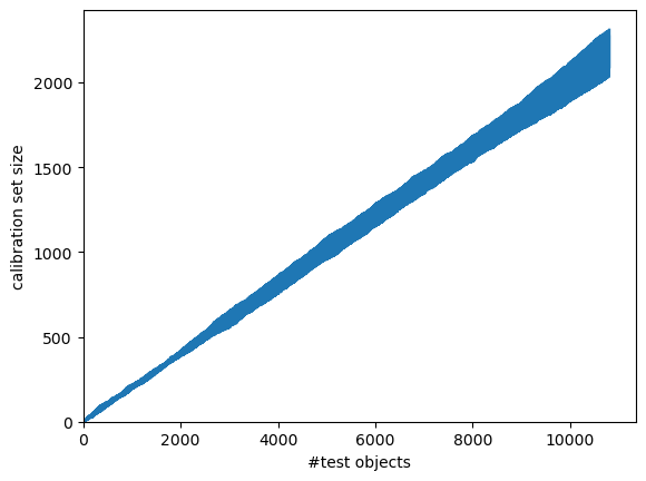
We may also evaluate the conformal predictive sytems using online calibration, by specifying online=True for the evaluate method (note that the metric “CRPS” is not available for semi-online conformal predictive systems):
[162]:
cps_std.evaluate(y_hat_test, y_test,
confidence=0.99, y_min=0, y_max=1,
online=True)
[162]:
{'error': 0.010086055334505462,
'eff_mean': 0.13482787103681543,
'eff_med': 0.13750077980327854,
'time_fit': 0.00018668174743652344,
'ks_test': 0.5006565865237772,
'time_evaluate': 0.24278593063354492}
[163]:
cps_norm.evaluate(y_hat_test, y_test,
sigmas=sigmas_test_var,
confidence=0.99, y_min=0, y_max=1,
online=True)
[163]:
{'error': 0.008790598686036821,
'eff_mean': 0.08393602252780262,
'eff_med': 0.060745501012132566,
'time_fit': 0.00023412704467773438,
'ks_test': 0.2779840566376811,
'time_evaluate': 0.24802398681640625}
[164]:
cps_mond_std.evaluate(y_hat_test, y_test,
bins=bins_test,
confidence=0.99, y_min=0, y_max=1,
online=True)
[164]:
{'error': 0.00925326177477559,
'eff_mean': 0.10201481540463607,
'eff_med': 0.06774775003278694,
'time_fit': 0.0008375644683837891,
'ks_test': 0.3284700751685238,
'time_evaluate': 0.16084742546081543}
[165]:
cps_mond_norm.evaluate(y_hat_test, y_test,
sigmas=sigmas_test_var,
bins=bins_test,
confidence=0.99, y_min=0, y_max=1,
online=True)
[165]:
{'error': 0.008513000832793605,
'eff_mean': 0.090107042458739,
'eff_med': 0.060465594345234366,
'time_fit': 0.00040149688720703125,
'ks_test': 0.3063346021509905,
'time_evaluate': 0.16530251502990723}
Again, we may consider ignoring the original calibration set by setting warm_start=False:
[166]:
cps_std.evaluate(y_hat_test, y_test,
confidence=0.99, y_min=0, y_max=1,
online=True, warm_start=False)
[166]:
{'error': 0.009808457481262134,
'eff_mean': 0.15125642618140295,
'eff_med': 0.13780128760655716,
'time_fit': 0.00018668174743652344,
'ks_test': 0.4949434902486165,
'time_evaluate': 0.23838019371032715}
[167]:
cps_norm.evaluate(y_hat_test, y_test,
sigmas=sigmas_test_var,
confidence=0.99, y_min=0, y_max=1,
online=True, warm_start=False)
[167]:
{'error': 0.010271120570000902,
'eff_mean': 0.09805686305991199,
'eff_med': 0.05871869158026194,
'time_fit': 0.00023412704467773438,
'ks_test': 0.276690739673481,
'time_evaluate': 0.24439716339111328}
[168]:
cps_mond_std.evaluate(y_hat_test, y_test,
bins=bins_test,
confidence=0.99, y_min=0, y_max=1,
online=True, warm_start=False)
[168]:
{'error': 0.007402609419820516,
'eff_mean': 0.1864993086527585,
'eff_med': 0.07864688708196721,
'time_fit': 0.0008375644683837891,
'ks_test': 0.30986167545420196,
'time_evaluate': 0.16988039016723633}
[169]:
cps_mond_norm.evaluate(y_hat_test, y_test,
sigmas=sigmas_test_var,
bins=bins_test,
confidence=0.99, y_min=0, y_max=1,
online=True, warm_start=False)
[169]:
{'error': 0.007495142037568292,
'eff_mean': 0.17315850597079538,
'eff_med': 0.06471947305032398,
'time_fit': 0.00040149688720703125,
'ks_test': 0.30739839927094925,
'time_evaluate': 0.16964149475097656}
Online calibration without an initial calibration set#
Since the calibration set is incrementally extended during online calibration, we may consider starting with an empty calibration set; this allows us to use the full training set when fitting the underlying model.
[170]:
rf_full = RandomForestRegressor(n_jobs=-1, n_estimators=500)
rf_full.fit(X_train, y_train)
[170]:
RandomForestRegressor(n_estimators=500, n_jobs=-1)In a Jupyter environment, please rerun this cell to show the HTML representation or trust the notebook.
On GitHub, the HTML representation is unable to render, please try loading this page with nbviewer.org.
Parameters
| n_estimators | 500 | |
| criterion | 'squared_error' | |
| max_depth | None | |
| min_samples_split | 2 | |
| min_samples_leaf | 1 | |
| min_weight_fraction_leaf | 0.0 | |
| max_features | 1.0 | |
| max_leaf_nodes | None | |
| min_impurity_decrease | 0.0 | |
| bootstrap | True | |
| oob_score | False | |
| n_jobs | -1 | |
| random_state | None | |
| verbose | 0 | |
| warm_start | False | |
| ccp_alpha | 0.0 | |
| max_samples | None | |
| monotonic_cst | None |
Let us compute non-conformity scores for the test set using the model trained on the full training set:
[171]:
y_hat_full = rf_full.predict(X_test)
We may now create a conformal predictive system, but this time without fitting a calibration set:
[172]:
cps_full = ConformalPredictiveSystem()
We may now obtain prediction intervals while sequentially updating the calibration set:
[173]:
cps_full.predict_int_online(y_hat_full, y_test, confidence=0.9)
[173]:
array([[ -inf, inf],
[ -inf, inf],
[ -inf, inf],
...,
[0.02422504, 0.06704088],
[0.02619799, 0.06901383],
[0.00687589, 0.04969173]])
If we provide also difficulty estimates (sigmas), we will obtain a normalized conformal predictive system:
[174]:
cps_full.predict_int_online(y_hat_full, y_test, sigmas=sigmas_test_var, confidence=0.9)
[174]:
array([[ -inf, inf],
[ -inf, inf],
[ -inf, inf],
...,
[0.03223534, 0.05761859],
[0.03412004, 0.05968652],
[0.01443343, 0.04075681]])
We get a Mondrian conformal predictive system by providing the categories for the test set, here by dividing the predictions into seven intervals:
[175]:
bin_thresholds = [0.0, 0.02, 0.04, 0.06, 0.08, 0.1, 0.5, 1.0]
bins_test = binning(rf_full.predict(X_test), bin_thresholds)
cps_full.predict_int_online(y_hat_full, y_test, bins=bins_test, confidence=0.9)
[175]:
array([[ -inf, inf],
[ -inf, inf],
[ -inf, inf],
...,
[0.02988368, 0.05935408],
[0.03185662, 0.06132703],
[0.01557903, 0.03666929]])
Let us investigate the coverage and prediction interval size for each category:
[176]:
intervals = cps_full.predict_int_online(y_hat_full, y_test,
bins=bins_test, y_min=0, y_max=1,
confidence=0.9)
number = []
coverage = []
size = []
for c in range(len(bin_thresholds)-1):
selection = bins_test == c
number.append(np.sum(selection))
coverage.append(np.sum(
(intervals[selection,0] <= y_test[selection])& \
(y_test[selection] <= intervals[selection,1]))/np.sum(selection))
size.append(np.sum(intervals[selection,1]-\
intervals[selection,0])/np.sum(selection))
df = pd.DataFrame({"Number":number, "Coverage":coverage, "Size":size})
df.round(4)
[176]:
| Number | Coverage | Size | |
|---|---|---|---|
| 0 | 594 | 0.9192 | 0.0533 |
| 1 | 3195 | 0.8958 | 0.0269 |
| 2 | 2833 | 0.9100 | 0.0378 |
| 3 | 1867 | 0.9020 | 0.0495 |
| 4 | 1036 | 0.8996 | 0.0711 |
| 5 | 1278 | 0.9030 | 0.1525 |
| 6 | 4 | 1.0000 | 1.0000 |
We can use predict_p_online to get the p-values:
[177]:
p_values = cps_full.predict_p_online(y_hat_test, y_test, bins=bins_test)
display(p_values)
plt.ecdf(p_values)
plt.xlim(0,1)
plt.xlabel("p-value")
plt.ylabel("ECDF")
plt.show()
print(f"KS-test: {kstest(p_values, "uniform").pvalue}")
array([0.57950871, 0.26996558, 0.82426319, ..., 0.09726203, 0.42172237,
0.41659263])
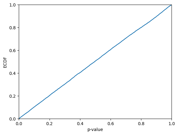
KS-test: 0.5739354899939673
We may get percentiles from the Mondrian conformal predictive system:
[178]:
cps_full.predict_percentiles_online(y_hat_test, y_test,
bins=bins_test,
lower_percentiles = [2.5, 25],
higher_percentiles = [50, 75, 97.5],
y_min=0, y_max=1)
[178]:
array([[0. , 0. , 1. , 1. , 1. ],
[0. , 0. , 1. , 1. , 1. ],
[0. , 0. , 1. , 1. , 1. ],
...,
[0.02591194, 0.03974367, 0.04439959, 0.04952501, 0.06645227],
[0.02786835, 0.04170008, 0.04636867, 0.05148869, 0.06840868],
[0.0128455 , 0.02343691, 0.02716481, 0.03039719, 0.04054171]])
We can of course also request the cpds; here we take a close look at those belonging to category 5:
[179]:
cpds = cps_full.predict_cpds_online(y_hat_test, y_test, bins=bins_test)
cpds[bins_test == 5]
[179]:
array([array([], dtype=float64), array([0.01898937]),
array([-0.00709527, 0.1103088 ]), ...,
array([-0.06031299, -0.04016145, -0.03736353, ..., 0.31366824,
0.31999868, 0.44570178]) ,
array([-0.06614302, -0.04599149, -0.04319356, ..., 0.3078382 ,
0.31416865, 0.43987174]) ,
array([-0.06585398, -0.04570244, -0.04290452, ..., 0.30812725,
0.31445769, 0.44016079]) ],
dtype=object)
We may also evaluate the conformal predictive system using online calibration, by specifying online=True for the evaluate method:
[180]:
cps_full.evaluate(y_hat_full, y_test, y_min=0, y_max=1, confidence=0.9,
online=True)
[180]:
{'error': 0.10280373831775702,
'eff_mean': 0.04370805382267408,
'eff_med': 0.04251358059016389,
'time_fit': None,
'ks_test': 0.8420509905644462,
'time_evaluate': 0.2842528820037842}
For Mondrian conformal predictive systems, we just have to provide the categories:
[181]:
cps_full.evaluate(y_hat_full, y_test, bins=bins_test, y_min=0, y_max=1,
confidence=0.9, online=True)
[181]:
{'error': 0.09688165078190059,
'eff_mean': 0.05456331575411808,
'eff_med': 0.03078541744262269,
'time_fit': None,
'ks_test': 0.823779336695137,
'time_evaluate': 0.14470314979553223}