Wrapping Classifiers and Regressors#
Importing packages#
In the examples below, we will be using the classes WrapClassifier and WrapRegressor from the crepes package. These classes rely on the classes ConformalClassifier, ConformalRegressor, and ConformalPredictiveSystem from the same package, which however will not be explicitly interfaced in the examples here; see here for how to obtain the same results as in this section by using these classes instead. The examples
below also use helper classes and functions from crepes.extras, as well as the NumPy, pandas, matplotlib and sklearn libraries.
[1]:
import numpy as np
import pandas as pd
import matplotlib.pyplot as plt

from sklearn.ensemble import RandomForestClassifier, RandomForestRegressor
from sklearn.model_selection import train_test_split
from sklearn.datasets import fetch_openml

from scipy.stats import kstest

from crepes import WrapClassifier, WrapRegressor, __version__

from crepes.extras import margin, DifficultyEstimator, MondrianCategorizer

print(f"crepes v. {__version__}")

np.random.seed(602211023)
np.set_printoptions(legacy='1.25')
crepes v. 0.9.1
Conformal classifiers#
Importing and splitting a classification dataset#
Let us import a classification dataset from www.openml.org.
[2]:
dataset = fetch_openml(name="gas-drift", parser="auto")

X = dataset.data.values.astype(float)
y = dataset.target.values
We now split the dataset into a training and a test set, and further split the training set into a proper training set and a calibration set.
[3]:
X_train, X_test, y_train, y_test = train_test_split(X, y, test_size=0.5)

X_prop_train, X_cal, y_prop_train, y_cal = train_test_split(X_train, y_train,
                                                            test_size=0.25)
Standard conformal classifier#
Let us create a standard conformal classifier through a WrapClassifier object, using a random forest that is fitted in the usual way (using the proper training set only), before or after being wrapped:
[4]:
rf = WrapClassifier(RandomForestClassifier(n_jobs=-1, n_estimators=500))

rf.fit(X_prop_train, y_prop_train)

display(rf)
WrapClassifier(learner=RandomForestClassifier(n_estimators=500, n_jobs=-1), calibrated=False)
We will use the the calibration set to calibrate the conformal regressor; note that the calibrate method has been added to the wrapped learner, in addition to the standard fitand predict methods.
[5]:
rf.calibrate(X_cal, y_cal)

display(rf)
WrapClassifier(learner=RandomForestClassifier(n_estimators=500, n_jobs=-1), calibrated=True, predictor=ConformalClassifier(fitted=True, mondrian=False))
We may now obtain prediction sets for the test set using the new method predict_set; here using the default confidence level (95%).
[6]:
prediction_sets = rf.predict_set(X_test)

display(prediction_sets[:20])
[['1'],
 ['2'],
 ['5'],
 ['2'],
 ['4'],
 ['6'],
 ['6'],
 ['1'],
 ['2'],
 ['6'],
 ['2'],
 ['2'],
 ['1'],
 ['2'],
 ['6'],
 [],
 [],
 ['6'],
 ['1'],
 ['5']]
We may alternatively represent each prediction set with a binary vector indicating the presence (1) or absence (0) of each class label by setting labels=False. The columns are ordered according to classes_ of the underlying learner:
[7]:
prediction_sets = rf.predict_set(X_test, labels=False)

display(prediction_sets[:20])
array([[1, 0, 0, 0, 0, 0],
       [0, 1, 0, 0, 0, 0],
       [0, 0, 0, 0, 1, 0],
       [0, 1, 0, 0, 0, 0],
       [0, 0, 0, 1, 0, 0],
       [0, 0, 0, 0, 0, 1],
       [0, 0, 0, 0, 0, 1],
       [1, 0, 0, 0, 0, 0],
       [0, 1, 0, 0, 0, 0],
       [0, 0, 0, 0, 0, 1],
       [0, 1, 0, 0, 0, 0],
       [0, 1, 0, 0, 0, 0],
       [1, 0, 0, 0, 0, 0],
       [0, 1, 0, 0, 0, 0],
       [0, 0, 0, 0, 0, 1],
       [0, 0, 0, 0, 0, 0],
       [0, 0, 0, 0, 0, 0],
       [0, 0, 0, 0, 0, 1],
       [1, 0, 0, 0, 0, 0],
       [0, 0, 0, 0, 1, 0]])
[8]:
rf.learner.classes_
[8]:
array(['1', '2', '3', '4', '5', '6'], dtype=object)
We may specify any confidence level that we are interested in, e.g., 99%. By increasing the confidence level, we can expect to see fewer labels getting rejected:
[9]:
prediction_sets = rf.predict_set(X_test, confidence=0.99)

display(prediction_sets[:20])
[['1'],
 ['2'],
 ['5'],
 ['2'],
 ['4'],
 ['6'],
 ['6'],
 ['1'],
 ['2'],
 ['6'],
 ['2'],
 ['2'],
 ['1'],
 ['2'],
 ['6'],
 ['2', '3'],
 ['5'],
 ['6'],
 ['1'],
 ['5']]
We may also get the p-values (without specifying any confidence level) by:
[10]:
p_values = rf.predict_p(X_test)

display(p_values)
array([[7.13862756e-02, 3.62010093e-04, 8.91455582e-04, 7.34373395e-03,
        1.91999540e-03, 2.07988781e-03],
       [2.40065581e-04, 4.01064413e-01, 3.40615569e-03, 2.38323560e-04,
        2.68620247e-04, 1.69191815e-03],
       [1.64313452e-03, 6.39837642e-04, 7.08056982e-04, 4.41564906e-04,
        7.57844073e-01, 1.61343588e-03],
       ...,
       [1.17526699e-03, 1.34252536e-03, 2.16860287e-03, 4.06163717e-03,
        3.27436288e-03, 2.06722834e-01],
       [2.02727275e-03, 1.86963492e-03, 1.73164894e-03, 7.29214810e-03,
        2.19183574e-03, 1.17842162e-01],
       [3.30268801e-03, 2.07926073e-03, 1.86262077e-03, 3.40122673e-03,
        7.74733743e-02, 7.36891399e-03]])
If we want only the p-values for the correct labels, we need to provide these and set all_classes=False:
[11]:
p_values = rf.predict_p(X_test, y_test, all_classes=False)
display(p_values)
array([0.06961041, 0.40808137, 0.75422722, ..., 0.20632515, 0.11800225,
       0.07668619])
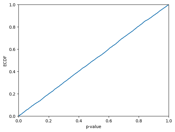
Let us take a look at how the p-values are distributed. From the visual inspection they may appear be approximaly uniformly distributed; this is however not guaranteed, since the p-values are not independent (see further below for semi-online conformal classifiers, for which this indeed holds). It is hence not very surprising if the Kolmogorov-Smirnov test allows us to reject that the p-values are sampled from a uniform distribution.
[12]:
plt.ecdf(p_values)
plt.xlim(0,1)
plt.xlabel("p-value")
plt.ylabel("ECDF")
plt.show()

print(f"KS-test: {kstest(p_values, "uniform").pvalue}")

KS-test: 0.0009057526555128788
By default, the conformal classifiers obtained using WrapClassifier will compute non-conformity scores using the hinge function defined in crepes.extras. We could alternatively generate a conformal classifier using the margin function, which we imported above:
[13]:
rf_margin = WrapClassifier(rf.learner)

rf_margin.calibrate(X_cal, y_cal, nc=margin)

display(rf_margin)
WrapClassifier(learner=RandomForestClassifier(n_estimators=500, n_jobs=-1), calibrated=True, predictor=ConformalClassifier(fitted=True, mondrian=False))
Mondrian conformal classifiers#
To control the error level across different groups of objects of interest, we may use so-called Mondrian conformal classifiers. A Mondrian conformal classifier if formed by providing a function or a MondrianCategorizer (defined in crepes.extras) as an additional argument, named mc, for the calibrate method.
For illustration, we will use the predicted labels of the underlying model to form the categories:
[14]:
rf_mond = WrapClassifier(rf.learner)
rf_mond.calibrate(X_cal, y_cal, mc=rf_mond.predict)

display(rf_mond)
WrapClassifier(learner=RandomForestClassifier(n_estimators=500, n_jobs=-1), calibrated=True, predictor=ConformalClassifier(fitted=True, mondrian=True))
We may now form prediction sets for the test objects (using the same categorization of the test objects under the hood):
[15]:
prediction_sets_mond = rf_mond.predict_set(X_test)

display(prediction_sets_mond[:20])
[[],
 ['2'],
 ['5'],
 ['2'],
 ['4'],
 ['6'],
 ['6'],
 ['1'],
 ['2'],
 ['6'],
 ['2'],
 ['2'],
 ['1'],
 ['2'],
 ['6'],
 [],
 [],
 ['6'],
 ['1'],
 ['5']]
We may also form the categories using a MondrianCategorizer, which may be fitted in several different ways. Below we show how to form categories by (equal-sized) binning of the first feature value, using five bins (instead of the default which is 10); note that we need objects to get the threshold values for the categories (bins):
[16]:
def get_values(X):
    return X[:,0]

mc_scoring = MondrianCategorizer()
mc_scoring.fit(X_cal, f=get_values, no_bins=5)

display(mc_scoring)
rf_mond_scoring = WrapClassifier(rf.learner)
rf_mond_scoring.calibrate(X_cal, y_cal, mc=mc_scoring)

display(rf_mond_scoring)
MondrianCategorizer(fitted=True, f=get_values, no_bins=5)
WrapClassifier(learner=RandomForestClassifier(n_estimators=500, n_jobs=-1), calibrated=True, predictor=ConformalClassifier(fitted=True, mondrian=True))
We may now form prediction sets for the test objects, again using the same Mondrian categorizer:
[17]:
prediction_sets_mond_scoring = rf_mond_scoring.predict_set(X_test)

display(prediction_sets_mond_scoring[:20])
[['1'],
 ['2'],
 ['5'],
 ['2'],
 ['4'],
 ['6'],
 ['6'],
 ['1'],
 ['2'],
 ['6'],
 ['2'],
 ['2'],
 ['1'],
 ['2'],
 ['6'],
 [],
 [],
 ['6'],
 ['1'],
 ['5']]
Class-conditional conformal classifiers#
Class-conditional conformal classifiers is a special type of Mondrian conformal classifiers where the categories are defined by actual (and not predicted, as above) class labels. The test objects need special treatment since we do not know to which categories they belong; a non-conformity score (p-value) is generated for each possible class label. Since this is a common type of conformal classifier, and it is a bit tricky to handle the test objects in the above way, the calibrate method has
a specific option (class_cond) to enable it, as shown below:
[18]:
rf_class_cond = WrapClassifier(rf.learner)

rf_class_cond.calibrate(X_cal, y_cal, class_cond=True)

display(rf_class_cond)
WrapClassifier(learner=RandomForestClassifier(n_estimators=500, n_jobs=-1), calibrated=True, predictor=ConformalClassifier(fitted=True, mondrian=True))
The prediction sets for the test objects are generated in the usual way:
[19]:
prediction_sets_class_cond = rf_class_cond.predict_set(X_test)

display(prediction_sets_class_cond[:20])
[['1'],
 ['2'],
 ['5'],
 ['2'],
 ['4'],
 ['6'],
 ['6'],
 ['1'],
 ['2'],
 ['6'],
 ['2'],
 ['2'],
 ['1'],
 ['2'],
 ['6'],
 [],
 [],
 ['6'],
 ['1'],
 ['5']]
Evaluating the conformal classifiers#
Since we have access to the correct class labels for the test set, we can investigate the predictive performance of the conformal classifiers. Let us start with the standard conformal classifier (which uses the default hinge function to compute non-conformity scores):
[20]:
rf.evaluate(X_test, y_test)
[20]:
{'error': 0.0404025880661395,
 'avg_c': 0.9610352264557872,
 'one_c': 0.9610352264557872,
 'empty': 0.038964773544212794,
 'ks_test': 0.0014393522574334269,
 'time_fit': 2.6226043701171875e-06,
 'time_evaluate': 0.6584126949310303}
Above we used the default (95%) confidence level, but we could specify some other:
[21]:
rf.evaluate(X_test, y_test, confidence=0.9)
[21]:
{'error': 0.0846872753414809,
 'avg_c': 0.9164629762760604,
 'one_c': 0.9164629762760604,
 'empty': 0.08353702372393962,
 'ks_test': 0.0011646076891647535,
 'time_fit': 2.6226043701171875e-06,
 'time_evaluate': 0.5932941436767578}
Let us also evaluate the standard conformal classifier that uses the margin function to compute non-conformity scores:
[22]:
rf_margin.evaluate(X_test, y_test, confidence=0.9)
[22]:
{'error': 0.08454349388928828,
 'avg_c': 0.9166067577282531,
 'one_c': 0.9166067577282531,
 'empty': 0.08339324227174695,
 'ks_test': 0.001609023552725607,
 'time_fit': 2.1457672119140625e-06,
 'time_evaluate': 0.8452470302581787}
The evaluation of the two Mondrian conformal classifiers (for which we used two different Mondrian categorizers) is done in the same way:
[23]:
rf_mond.evaluate(X_test, y_test, confidence=0.9)
[23]:
{'error': 0.08856937455068292,
 'avg_c': 0.9125808770668584,
 'one_c': 0.9125808770668584,
 'empty': 0.08741912293314162,
 'ks_test': 4.6570300579077785e-05,
 'time_fit': 2.1457672119140625e-06,
 'time_evaluate': 0.620652437210083}
[24]:
rf_mond_scoring.evaluate(X_test, y_test, confidence=0.9)
[24]:
{'error': 0.08310567936736157,
 'avg_c': 0.917900790797987,
 'one_c': 0.917900790797987,
 'empty': 0.08209920920201294,
 'ks_test': 0.00011696311369026331,
 'time_fit': 2.6226043701171875e-06,
 'time_evaluate': 0.5084836483001709}
Let us also evaluate the class-conditional conformal classifier:
[25]:
rf_class_cond.evaluate(X_test, y_test, confidence=0.9)
[25]:
{'error': 0.09158878504672896,
 'avg_c': 0.9094176851186196,
 'one_c': 0.9094176851186196,
 'empty': 0.0905823148813803,
 'ks_test': 0.00010233707244509156,
 'time_fit': 4.76837158203125e-07,
 'time_evaluate': 2.1958987712860107}
We may evaluate the conformal classifiers on each class separately. For the standard conformal classifier, we get:
[26]:
for c in rf.learner.classes_:
    print(f"Class {c}:")
    display(rf.evaluate(X_test[y_test == c], y_test[y_test == c], confidence=0.9))
    print("")
Class 1:
{'error': 0.06692607003891049,
 'avg_c': 0.9330739299610895,
 'one_c': 0.9330739299610895,
 'empty': 0.0669260700389105,
 'ks_test': 3.657970890101206e-10,
 'time_fit': 2.6226043701171875e-06,
 'time_evaluate': 0.17757964134216309}
Class 2:
{'error': 0.05842391304347827,
 'avg_c': 0.9429347826086957,
 'one_c': 0.9429347826086957,
 'empty': 0.057065217391304345,
 'ks_test': 1.3371766828562141e-55,
 'time_fit': 2.6226043701171875e-06,
 'time_evaluate': 0.19403457641601562}
Class 3:
{'error': 0.08222490931076176,
 'avg_c': 0.9238210399032648,
 'one_c': 0.9238210399032648,
 'empty': 0.0761789600967352,
 'ks_test': 0.0019542319244032972,
 'time_fit': 2.6226043701171875e-06,
 'time_evaluate': 0.1428816318511963}
Class 4:
{'error': 0.15583075335397312,
 'avg_c': 0.8441692466460269,
 'one_c': 0.8441692466460269,
 'empty': 0.15583075335397317,
 'ks_test': 7.89189148237677e-90,
 'time_fit': 2.6226043701171875e-06,
 'time_evaluate': 0.15318536758422852}
Class 5:
{'error': 0.07702612190221036,
 'avg_c': 0.9229738780977896,
 'one_c': 0.9229738780977896,
 'empty': 0.07702612190221031,
 'ks_test': 1.0723469629254118e-20,
 'time_fit': 2.6226043701171875e-06,
 'time_evaluate': 0.18946409225463867}
Class 6:
{'error': 0.09240924092409242,
 'avg_c': 0.9086908690869087,
 'one_c': 0.9086908690869087,
 'empty': 0.09130913091309131,
 'ks_test': 1.231680396534135e-44,
 'time_fit': 2.6226043701171875e-06,
 'time_evaluate': 0.1482694149017334}
As can be observed above, a standard conformal classifier may significantly exceed the error level when considering each class separately. This contrasts to the class-condition conformal classifier:
[27]:
for c in rf.learner.classes_:
    print(f"Class {c}:")
    display(rf_class_cond.evaluate(X_test[y_test == c], y_test[y_test == c], confidence=0.9))
    print("")
Class 1:
{'error': 0.09105058365758756,
 'avg_c': 0.9089494163424124,
 'one_c': 0.9089494163424124,
 'empty': 0.09105058365758754,
 'ks_test': 0.00032185876891012183,
 'time_fit': 4.76837158203125e-07,
 'time_evaluate': 0.48041224479675293}
Class 2:
{'error': 0.10665760869565222,
 'avg_c': 0.8947010869565217,
 'one_c': 0.8947010869565217,
 'empty': 0.10529891304347826,
 'ks_test': 0.06992776631843445,
 'time_fit': 4.76837158203125e-07,
 'time_evaluate': 0.5231339931488037}
Class 3:
{'error': 0.09915356711003631,
 'avg_c': 0.905683192261185,
 'one_c': 0.905683192261185,
 'empty': 0.094316807738815,
 'ks_test': 0.04644994758969123,
 'time_fit': 4.76837158203125e-07,
 'time_evaluate': 0.32725071907043457}
Class 4:
{'error': 0.0980392156862745,
 'avg_c': 0.9019607843137255,
 'one_c': 0.9019607843137255,
 'empty': 0.09803921568627451,
 'ks_test': 0.007728310905532813,
 'time_fit': 4.76837158203125e-07,
 'time_evaluate': 0.37015509605407715}
Class 5:
{'error': 0.09042196918955125,
 'avg_c': 0.9095780308104487,
 'one_c': 0.9095780308104487,
 'empty': 0.09042196918955124,
 'ks_test': 5.94729336717876e-05,
 'time_fit': 4.76837158203125e-07,
 'time_evaluate': 0.5211069583892822}
Class 6:
{'error': 0.0517051705170517,
 'avg_c': 0.9493949394939494,
 'one_c': 0.9493949394939494,
 'empty': 0.050605060506050605,
 'ks_test': 0.0006589488221906246,
 'time_fit': 4.76837158203125e-07,
 'time_evaluate': 0.3561844825744629}
Semi-online conformal classifiers#
The above conformal classifiers are fitted once using the provided calibration set. In case we are receiving the correct label for each test object immediately after making a prediction, we may consider the option of employing online calibration, i.e., continuously updating the calibration set. This is done by setting online=True when calling the methods predict_p, predict_set, and evaluate.
Online calibration with an already calibrated conformal classifier#
Here we will obtain p-values computed in an online fashion for the above fitted standard conformal classifier. Note that in addition to the test objects, we also need to provide the correct labels.
[28]:
rf.predict_p(X_test, y_test, online=True)
[28]:
array([[7.05210250e-02, 2.20442066e-04, 7.66373791e-04, 6.90757217e-03,
        2.08178316e-03, 1.91601673e-03],
       [7.07172362e-05, 4.03048113e-01, 3.11648442e-03, 1.55416709e-03,
        8.55741026e-04, 1.48611069e-03],
       [5.06911880e-04, 1.25229229e-03, 2.54932077e-04, 6.78813798e-04,
        7.90077053e-01, 1.38401947e-03],
       ...,
       [4.56194929e-04, 4.07415133e-04, 5.73874047e-04, 2.11524754e-03,
        9.84585233e-04, 1.95011587e-01],
       [4.71684764e-04, 5.63336305e-04, 3.85153378e-04, 2.88403671e-03,
        4.84927297e-04, 1.11657775e-01],
       [9.86190594e-04, 4.73247018e-04, 5.44064322e-04, 1.08410491e-03,
        6.70129058e-02, 3.25803367e-03]])
[29]:
rf_class_cond.predict_p(X_test, y_test, online=True)
[29]:
array([[5.09135308e-02, 7.97588408e-04, 6.84361644e-03, 1.12331219e-02,
        4.03387190e-03, 2.11244950e-04],
       [2.07501525e-03, 2.37888234e-01, 1.23848370e-02, 3.09900384e-03,
        2.77899559e-03, 3.73854760e-03],
       [8.45071677e-04, 1.56290350e-03, 4.34628306e-03, 1.45791324e-03,
        7.00259691e-01, 1.62296386e-03],
       ...,
       [3.26370245e-04, 4.74349515e-04, 3.58174385e-03, 4.02266599e-03,
        5.69384302e-04, 2.97936666e-01],
       [4.09288533e-04, 4.00073308e-04, 3.34187579e-03, 4.04472205e-03,
        7.28106257e-04, 1.37948700e-01],
       [3.13109054e-04, 2.58215940e-04, 3.26647966e-03, 2.31159795e-03,
        6.74177987e-02, 2.11417717e-03]])
Similarly, we can obtain prediction sets based on the p-values computed online, which are compared to the specified level of confidence:
[30]:
online_prediction_sets = rf_mond.predict_set(X_test, y_test, confidence=0.99, online=True)
online_prediction_sets[:20]
[30]:
[['1'],
 ['2'],
 ['5'],
 ['2'],
 ['4'],
 ['6'],
 ['6'],
 ['1'],
 ['2'],
 ['4', '6'],
 ['2'],
 ['2'],
 ['1'],
 ['2'],
 ['4', '6'],
 ['2', '3'],
 ['4', '5', '6'],
 ['6'],
 ['1'],
 ['5']]
[31]:
online_prediction_sets = rf_class_cond.predict_set(X_test, y_test, confidence=0.99, online=True)
online_prediction_sets[:20]
[31]:
[['1', '4'],
 ['2', '3'],
 ['5'],
 ['2', '3'],
 ['3', '4'],
 ['6'],
 ['6'],
 ['1'],
 ['2'],
 ['3', '6'],
 ['2'],
 ['2', '3'],
 ['1'],
 ['2'],
 ['6'],
 ['3'],
 ['3', '4'],
 ['6'],
 ['1'],
 ['5']]
By default, the test objects and labels are sequentially added to the existing calibration set, i.e., the one used when calibrating the conformal classifier. If we would like the original calibration set to be ignored, we can set the warm_start option to False. Note that few (if any) class labels will be excluded from the initial prediction sets, before we have a sufficiently large calibration set to allow for excluding labels at the specified level of confidence.
[32]:
online_prediction_sets = rf_mond.predict_set(X_test, y_test, confidence=0.99,
                                             online=True, warm_start=False)
display(online_prediction_sets[:10])
print("...")
display(online_prediction_sets[-10:])
[['1', '2', '3', '4', '5', '6'],
 ['1', '2', '3', '4', '5', '6'],
 ['1', '2', '3', '4', '5', '6'],
 ['1', '2', '3', '4', '5', '6'],
 ['1', '2', '3', '4', '5', '6'],
 ['1', '2', '3', '4', '5', '6'],
 ['1', '2', '3', '4', '5', '6'],
 ['1', '2', '3', '4', '5', '6'],
 ['1', '2', '3', '4', '5', '6'],
 ['1', '2', '3', '4', '5', '6']]
...
[['2'], ['4'], ['6'], ['2'], ['4'], ['5'], ['4'], ['6'], ['6'], ['5']]
[33]:
online_prediction_sets = rf_class_cond.predict_set(X_test, y_test, confidence=0.99,
                                                   online=True, warm_start=False)

display(online_prediction_sets[:10])
print("...")
display(online_prediction_sets[-10:])
[['1', '2', '3', '4', '5', '6'],
 ['1', '2', '3', '4', '5', '6'],
 ['1', '2', '3', '4', '5', '6'],
 ['1', '2', '3', '4', '5', '6'],
 ['1', '2', '3', '4', '5'],
 ['1', '2', '3', '4', '5', '6'],
 ['1', '2', '3', '4', '5', '6'],
 ['1', '2', '3', '4', '5', '6'],
 ['1', '2', '3', '4', '5', '6'],
 ['1', '2', '3', '4', '5', '6']]
...
[['2'], ['4'], ['6'], ['2'], ['4'], ['5'], ['4'], ['6'], ['6'], ['5']]
Let us take a look at how the p-values for the correct labels are distributed. From both the visual inspection and the Kolmogorov-Smirnov test, we cannot rule out that the p-values are sampled from a uniform distribution.
[34]:
p_values = rf_class_cond.predict_p(X_test, y_test, all_classes=False,
                                    online=True, warm_start=False)

plt.ecdf(p_values)
plt.xlim(0,1)
plt.xlabel("p-value")
plt.ylabel("ECDF")
plt.show()

print(f"KS-test: {kstest(p_values, "uniform").pvalue}")
KS-test: 0.4501896231006376
We may also evaluate the conformal classifiers using online calibration, by specifying online=True for the evaluate method:
[35]:
rf_mond.evaluate(X_test, y_test, confidence=0.99, online=True)
[35]:
{'error': 0.007764198418404034,
 'avg_c': 1.0178289000718908,
 'one_c': 0.9794392523364486,
 'empty': 0.003882099209202013,
 'ks_test': 0.11932891556937242,
 'time_fit': 2.1457672119140625e-06,
 'time_evaluate': 0.6959662437438965}
[36]:
rf_class_cond.evaluate(X_test, y_test, confidence=0.99, online=True)
[36]:
{'error': 0.007764198418404034,
 'avg_c': 1.0277498202731847,
 'one_c': 0.9652048885693746,
 'empty': 0.003882099209202013,
 'ks_test': 0.08920155399189122,
 'time_fit': 4.76837158203125e-07,
 'time_evaluate': 0.6218359470367432}
Again, we may consider ignoring the original calibration set by setting warm_start=False:
[37]:
rf_mond.evaluate(X_test, y_test, confidence=0.99, online=True, warm_start=False)
[37]:
{'error': 0.009777138749101355,
 'avg_c': 1.2182602444284687,
 'one_c': 0.913587347232207,
 'empty': 0.005463695183321351,
 'ks_test': 0.8759425945392264,
 'time_fit': 2.1457672119140625e-06,
 'time_evaluate': 0.7845466136932373}
Online calibration without an initial calibration set#
Since the calibration set is incrementally extended during online calibration, we may consider starting with an empty calibration set; this allows us to use the full training set when fitting the underlying model.
[38]:
rf_full = WrapClassifier(RandomForestClassifier(n_jobs=-1, n_estimators=500))

rf_full.fit(X_train, y_train)
Let us first initialize the conformal classifier with an empty calibration set, i.e., not specifying any objects or labels for the calibrate method (we may still provide a non-conformity function and Mondrian categorizer):
[39]:
rf_full.calibrate()
[39]:
WrapClassifier(learner=RandomForestClassifier(n_estimators=500, n_jobs=-1), calibrated=False)
We may now obtain prediction sets while sequentially adding test objects and labels to the calibration set:
[40]:
prediction_sets_online = rf_full.predict_set(X_test, y_test, confidence=0.99, online=True)

display(prediction_sets_online[:40])
[['1', '2', '3', '4', '5', '6'],
 ['1', '2', '3', '4', '5', '6'],
 ['1', '2', '3', '4', '5', '6'],
 ['1', '2', '3', '4', '5', '6'],
 ['1', '2', '3', '4', '5', '6'],
 ['1', '2', '3', '4', '5', '6'],
 ['1', '2', '4', '5', '6'],
 ['1', '3', '4', '5', '6'],
 ['2', '3', '4', '5', '6'],
 ['1', '2', '3', '4', '5', '6'],
 ['1', '2', '3', '4', '5', '6'],
 ['1', '2', '3', '4', '6'],
 ['1', '2', '4', '5', '6'],
 ['1', '2', '4', '5', '6'],
 ['1', '2', '3', '4', '5', '6'],
 ['1', '2', '3', '4', '5', '6'],
 ['1', '2', '3', '4', '5', '6'],
 ['1', '2', '3', '4', '5', '6'],
 ['1', '2', '3', '4', '5', '6'],
 ['1', '3', '4', '5', '6'],
 ['2', '3', '4', '5', '6'],
 ['1', '4', '5', '6'],
 ['1', '2', '3', '4', '5', '6'],
 ['1', '2', '3', '4', '6'],
 ['1', '2', '4', '5', '6'],
 ['1', '2', '3', '5', '6'],
 ['1', '2', '3', '4', '5', '6'],
 ['3', '4', '5', '6'],
 ['1', '2', '3', '4', '5', '6'],
 ['2', '3', '4', '5', '6'],
 ['2', '5'],
 ['1', '4', '5', '6'],
 ['1', '4', '5', '6'],
 ['4'],
 ['1', '2', '3', '4', '5', '6'],
 ['3', '4', '5', '6'],
 ['1', '2', '4', '5', '6'],
 ['1', '3', '4', '5', '6'],
 ['1', '2', '3', '4', '5'],
 ['1', '2', '3', '5', '6']]
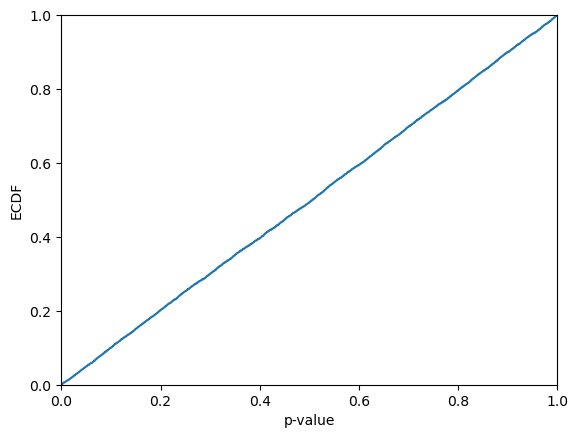
Let us take a look at how the p-values for the correct labels are distributed. From both the visual inspection and the Kolmogorov-Smirnov test, we cannot rule out that the p-values are sampled from a uniform distribution.
[41]:
p_values = rf_full.predict_p(X_test, y_test, all_classes=False, online=True)

plt.ecdf(p_values)
plt.xlim(0,1)
plt.xlabel("p-value")
plt.ylabel("ECDF")
plt.show()

print(f"KS-test: {kstest(p_values, "uniform").pvalue}")

KS-test: 0.5104542869586581
We may also evaluate the conformal classifier using online calibration, by specifying online=True for the evaluate method:
[42]:
rf_full.evaluate(X_test, y_test, confidence=0.99, online=True)
[42]:
{'error': 0.009777138749101355,
 'avg_c': 1.0277498202731847,
 'one_c': 0.9810208483105679,
 'empty': 0.007189072609633357,
 'ks_test': 0.5786730875007888,
 'time_fit': 4.76837158203125e-07,
 'time_evaluate': 0.7269594669342041}
Out-of-bag calibration#
For conformal classifiers that employ learners that use bagging, like random forests, we may consider an alternative strategy to dividing the original training set into a proper training and calibration set; we may use the out-of-bag (OOB) predictions, which allow us to use the full training set for both model building and calibration. It should be noted that this strategy does not come with the theoretical validity guarantee of the above (inductive) conformal classifiers, due to that calibration and test instances are not handled in exactly the same way. In practice, however, conformal classifiers based on out-of-bag predictions rarely fail to meet the coverage requirements.
Standard conformal classifiers with out-of-bag calibration#
Let us first generate a model from the full training set, making sure the learner has an attribute oob_decision_function_, which e.g. is the case for a RandomForestClassifier if oob_score is set to True when created.
[43]:
learner_full = RandomForestClassifier(n_jobs=-1, n_estimators=500, oob_score=True)

rf = WrapClassifier(learner_full)

rf.fit(X_train, y_train)
We may now obtain a standard conformal classifier using OOB predictions:
[44]:
rf.calibrate(X_train, y_train, oob=True)

display(rf)
WrapClassifier(learner=RandomForestClassifier(n_estimators=500, n_jobs=-1, oob_score=True), calibrated=True, predictor=ConformalClassifier(fitted=True, mondrian=False))
… and use it to get prediction sets for the test set:
[45]:
prediction_sets_oob = rf.predict_set(X_test)

display(prediction_sets_oob[:40])
[[],
 ['2'],
 ['5'],
 ['2'],
 ['4'],
 ['6'],
 ['6'],
 ['1'],
 ['2'],
 ['6'],
 ['2'],
 ['2'],
 ['1'],
 ['2'],
 ['6'],
 [],
 [],
 ['6'],
 ['1'],
 ['5'],
 ['5'],
 ['4'],
 ['4'],
 ['2'],
 ['1'],
 ['3'],
 ['1'],
 ['3'],
 ['2'],
 ['5'],
 ['2'],
 ['5'],
 ['1'],
 ['4'],
 ['4'],
 ['5'],
 ['5'],
 ['1'],
 ['2'],
 ['5']]
Mondrian conformal classifiers with out-of-bag calibration#
Using out-of-bag calibration works equally well for Mondrian conformal classifiers:
[46]:
rf.calibrate(X_train, y_train, mc=mc_scoring, oob=True)

display(rf)
WrapClassifier(learner=RandomForestClassifier(n_estimators=500, n_jobs=-1, oob_score=True), calibrated=True, predictor=ConformalClassifier(fitted=True, mondrian=True))
Prediction sets for the test objects are obtained in the usual way:
[47]:
prediction_sets_mond_oob = rf.predict_set(X_test)

display(prediction_sets_oob[:20])
[[],
 ['2'],
 ['5'],
 ['2'],
 ['4'],
 ['6'],
 ['6'],
 ['1'],
 ['2'],
 ['6'],
 ['2'],
 ['2'],
 ['1'],
 ['2'],
 ['6'],
 [],
 [],
 ['6'],
 ['1'],
 ['5']]
We may of course evaluate the Mondrian conformal classifier using out-of-bag predictions too:
[48]:
results = rf.evaluate(X_test, y_test, confidence=0.99)

display(results)
{'error': 0.007620416966211407,
 'avg_c': 1.0,
 'one_c': 0.9928109273903667,
 'empty': 0.0035945363048166786,
 'ks_test': 6.167896821085361e-19,
 'time_fit': 4.76837158203125e-07,
 'time_evaluate': 0.5840909481048584}
Class-conditional conformal classifiers with out-of-bag calibration#
Unsurprisingly, since a class-conditional conformal classifier is a special type of Mondrian conformal classifier, we can use out-of-bag calibration for them too:
[49]:
rf.calibrate(X_train, y_train, class_cond=True, oob=True)

display(rf)
WrapClassifier(learner=RandomForestClassifier(n_estimators=500, n_jobs=-1, oob_score=True), calibrated=True, predictor=ConformalClassifier(fitted=True, mondrian=True))
Prediction sets for the test objects are obtained in the usual way:
[50]:
prediction_sets_class_cond_oob = rf.predict_set(X_test)

display(prediction_sets_class_cond_oob[:20])
[[],
 ['2'],
 ['5'],
 ['2'],
 ['4'],
 ['6'],
 ['6'],
 ['1'],
 ['2'],
 ['6'],
 ['2'],
 ['2'],
 ['1'],
 ['2'],
 ['6'],
 [],
 [],
 ['6'],
 ['1'],
 ['5']]
Finally, for completeness, we show that a class-conditional conformal classifier formed using out-of-bag calibration may be evaluated too:
[51]:
results = rf.evaluate(X_test, y_test, confidence=0.99)

display(results)
{'error': 0.005895039539899338,
 'avg_c': 1.0071890726096333,
 'one_c': 0.9873472322070453,
 'empty': 0.0027318475916606757,
 'ks_test': 4.244385727983511e-25,
 'time_fit': 4.76837158203125e-07,
 'time_evaluate': 2.510770082473755}
Let us also check the performance for the classes separately:
[52]:
for c in rf.learner.classes_:
    print(f"Class {c}:")
    display(rf.evaluate(X_test[y_test == c], y_test[y_test == c], confidence=0.99))
    print("")
Class 1:
{'error': 0.006225680933852118,
 'avg_c': 0.9961089494163424,
 'one_c': 0.9945525291828794,
 'empty': 0.004669260700389105,
 'ks_test': 4.9044007419158925e-06,
 'time_fit': 4.76837158203125e-07,
 'time_evaluate': 0.5501096248626709}
Class 2:
{'error': 0.008831521739130488,
 'avg_c': 1.029211956521739,
 'one_c': 0.9667119565217391,
 'empty': 0.0020380434782608695,
 'ks_test': 1.8726080521071582e-09,
 'time_fit': 4.76837158203125e-07,
 'time_evaluate': 0.6172313690185547}
Class 3:
{'error': 0.006045949214026569,
 'avg_c': 1.0048367593712213,
 'one_c': 0.9951632406287787,
 'empty': 0.0,
 'ks_test': 1.0250290286256342e-09,
 'time_fit': 4.76837158203125e-07,
 'time_evaluate': 0.3952610492706299}
Class 4:
{'error': 0.00515995872033026,
 'avg_c': 1.0020639834881322,
 'one_c': 0.9917440660474717,
 'empty': 0.0030959752321981426,
 'ks_test': 0.0003866659183591781,
 'time_fit': 4.76837158203125e-07,
 'time_evaluate': 0.4297034740447998}
Class 5:
{'error': 0.002009377093101117,
 'avg_c': 1.0080375083724045,
 'one_c': 0.9879437374413932,
 'empty': 0.0020093770931011385,
 'ks_test': 9.468567001920994e-16,
 'time_fit': 4.76837158203125e-07,
 'time_evaluate': 0.6752974987030029}
Class 6:
{'error': 0.00990099009900991,
 'avg_c': 0.9944994499449945,
 'one_c': 0.9944994499449945,
 'empty': 0.005500550055005501,
 'ks_test': 0.014885745116550895,
 'time_fit': 4.76837158203125e-07,
 'time_evaluate': 0.4570741653442383}
Conformal regressors#
Importing and splitting a regression dataset#
Let us import a dataset from www.openml.org and min-max normalize the targets; the latter is not really necessary, but useful, allowing to directly compare the size of a prediction interval to the whole target range, which becomes 1.0 in this case.
[53]:
dataset = fetch_openml(name="house_sales", version=3, parser="auto")

X = dataset.data.values.astype(float)
y = dataset.target.values.astype(float)

y = np.array([(y[i]-y.min())/(y.max()-y.min()) for i in range(len(y))])
We now split the dataset into a training and a test set, and further split the training set into a proper training set and a calibration set.
[54]:
X_train, X_test, y_train, y_test = train_test_split(X, y, test_size=0.5)

X_prop_train, X_cal, y_prop_train, y_cal = train_test_split(X_train, y_train,
                                                            test_size=0.25)
Standard conformal regressors#
Let us create a conformal regressor through a WrapRegressor object, using a random forest that is fitted in the usual way (using the proper training set only), before or after being wrapped:
[55]:
rf = WrapRegressor(RandomForestRegressor(n_jobs=-1, n_estimators=500, oob_score=True))

rf.fit(X_prop_train, y_prop_train)

display(rf)
WrapRegressor(learner=RandomForestRegressor(n_estimators=500, n_jobs=-1, oob_score=True), calibrated=False)
We will use the the calibration set to calibrate the conformal regressor; note that the calibrate method has been added to the wrapped learner, in addition to the standard fitand predict methods.
[56]:
rf.calibrate(X_cal, y_cal)

display(rf)
WrapRegressor(learner=RandomForestRegressor(n_estimators=500, n_jobs=-1, oob_score=True), calibrated=True, predictor=ConformalRegressor(fitted=True, normalized=False, mondrian=False))
We may now obtain prediction intervals for the test set using the new method predict_int; here using a confidence level of 99%.
[57]:
intervals = rf.predict_int(X_test, confidence=0.99)

display(intervals)
array([[-0.04922302,  0.09725752],
       [-0.00660463,  0.13987591],
       [-0.00814742,  0.13833312],
       ...,
       [ 0.10741278,  0.25389333],
       [-0.05339337,  0.09308717],
       [ 0.00437286,  0.1508534 ]])
We may request that the intervals are cut to exclude impossible values, in this case below 0 and above 1; below we also use the default confidence level (95%), which further tightens the intervals.
[58]:
intervals_std = rf.predict_int(X_test, y_min=0, y_max=1)

display(intervals_std)
array([[0.        , 0.05344703],
       [0.03720586, 0.09606542],
       [0.03566307, 0.09452263],
       ...,
       [0.15122328, 0.21008283],
       [0.        , 0.04927668],
       [0.04818335, 0.10704291]])
If we want to obtain the p-values for the correct labels, we can use predict_p, and in addition to the point predictions also provide the correct labels:
[59]:
p_values = rf.predict_p(X_test, y_test)
display(p_values)
array([0.52842524, 0.06623902, 0.1704223 , ..., 0.08864116, 0.23583885,
       0.72024669])
Let us take a look at how the p-values are distributed. From the visual inspection they may appear be approximaly uniformly distributed; this is however not guaranteed, since the p-values are not independent (see further below for semi-online conformal regressors, for which this indeed holds). It is hence not very surprising if the Kolmogorov-Smirnov test allows us to reject that the p-values are sampled from a uniform distribution.
[60]:
plt.ecdf(p_values)
plt.xlim(0,1)
plt.xlabel("p-value")
plt.ylabel("ECDF")
plt.show()

print(f"KS-test: {kstest(p_values, "uniform").pvalue}")

KS-test: 0.00293454244196997
Accessing the wrapped learner#
As shown above, we have access directly to some methods of the wrapped learner, e.g., through the fit and predict methods. We can also access the wrapped learner directly by the following:
[61]:
learner_prop = rf.learner
This may be useful, e.g., in case a fitted wrapped learner is to be re-used in another conformal regressor, as we will see below.
Normalized conformal regressors#
The above intervals are not normalized, i.e., they are all of the same size (at least before they are cut). We could make the intervals more informative through normalization using difficulty estimates; more difficult instances will be assigned wider intervals. We can use a DifficultyEstimator, as imported from crepes.extras, for this purpose. It can be used to estimate the difficulty by using k-nearest neighbors in three different ways: i) by the (Euclidean) distances to the nearest
neighbors, ii) by the standard deviation of the targets of the nearest neighbors, and iii) by the absolute errors of the k nearest neighbors.
A small value (beta) is added to the estimates, which may be given through a (named) argument to the fit method; we will just use the default for this, i.e., beta=0.01. In order to make the beta value have the same effect across different estimators, we may opt for normalizing the difficulty estimates (using min-max scaling) by setting scaler=True. It should be noted that this comes with a computational cost; for estimators based on the k-nearest neighbor, a leave-one-out protocol is
employed to find the minimum and maximum distances that are used by the scaler.
We will first consider just using the first option (distances to the k-nearest neighbors) to produce normalized conformal regressors, using the default number of nearest neighbors, i.e., k=25.
[62]:
de_knn = DifficultyEstimator()

de_knn.fit(X=X_prop_train, scaler=True)

display(de_knn)
DifficultyEstimator(fitted=True, type=knn, k=25, target=none, scaler=True, beta=0.01, oob=False)
We create a new (normalized) conformal regressor re-using the underlying (already fitted) learner of the previous conformal regressor, and calibrate it using the calibration objects and labels together the difficulty estimator:
[63]:
rf_norm_knn_dist = WrapRegressor(learner_prop)

rf_norm_knn_dist.calibrate(X_cal, y_cal, de=de_knn)

display(rf_norm_knn_dist)
WrapRegressor(learner=RandomForestRegressor(n_estimators=500, n_jobs=-1, oob_score=True), calibrated=True, predictor=ConformalRegressor(fitted=True, normalized=True, mondrian=False))
To obtain prediction intervals, we just have to provide test objects to the predict_int method, as the difficulty estimates will be computed by the incorporated difficulty estimator:
[64]:
intervals_norm_knn_dist = rf_norm_knn_dist.predict_int(X_test, y_min=0, y_max=1)

display(intervals_norm_knn_dist)
array([[0.01097246, 0.03706205],
       [0.04218894, 0.09108234],
       [0.03782359, 0.09236211],
       ...,
       [0.11921407, 0.24209204],
       [0.00350158, 0.03619222],
       [0.04768591, 0.10754034]])
Alternatively, we could estimate the difficulty using the standard deviation of the targets of the nearest neighbors; we specify this by providing the targets too to the fit method:
[65]:
de_knn_std = DifficultyEstimator()

de_knn_std.fit(X=X_prop_train, y=y_prop_train, scaler=True)

display(de_knn_std)

rf_norm_knn_std = WrapRegressor(learner_prop)

rf_norm_knn_std.calibrate(X_cal, y_cal, de=de_knn_std)

display(rf_norm_knn_std)
DifficultyEstimator(fitted=True, type=knn, k=25, target=labels, scaler=True, beta=0.01, oob=False)
WrapRegressor(learner=RandomForestRegressor(n_estimators=500, n_jobs=-1, oob_score=True), calibrated=True, predictor=ConformalRegressor(fitted=True, normalized=True, mondrian=False))
We obtain the prediction intervals in the same way as before:
[66]:
intervals_norm_knn_std = rf_norm_knn_std.predict_int(X_test, y_min=0, y_max=1)

display(intervals_norm_knn_std)
array([[0.01461994, 0.03341457],
       [0.02832566, 0.10494562],
       [0.04462997, 0.08555573],
       ...,
       [0.11989873, 0.24140738],
       [0.01363883, 0.02605498],
       [0.05935098, 0.09587527]])
A third option is to use (absolute) residuals for the reference objects. For a model that overfits the training data, it can be a good idea to use a separate set of (reference) objects and labels from which the residuals could be calculated, rather than using the original training data. Since we in this case have trained a random forest, we opt for estimating the residuals by using the out-of-bag predictions for the training instances, where the latter are stored in oob_prediction_ of the
underlying lerner (as a consequence of setting oob_score=True for the RandomForestRegressor above.)
To inform the fit method that this is what we want to do, we provide a value for residuals, instead of y as we did above for the option to use the (standard deviation of) the targets.
[67]:
residuals_prop_oob = y_prop_train - rf.learner.oob_prediction_

de_knn_res = DifficultyEstimator()

de_knn_res.fit(X=X_prop_train, residuals=residuals_prop_oob, scaler=True)

display(de_knn_res)

rf_norm_knn_res = WrapRegressor(learner_prop)

rf_norm_knn_res.calibrate(X_cal, y_cal, de=de_knn_res)

display(rf_norm_knn_res)
DifficultyEstimator(fitted=True, type=knn, k=25, target=residuals, scaler=True, beta=0.01, oob=False)
WrapRegressor(learner=RandomForestRegressor(n_estimators=500, n_jobs=-1, oob_score=True), calibrated=True, predictor=ConformalRegressor(fitted=True, normalized=True, mondrian=False))
Let us also generate the prediction intervals:
[68]:
intervals_norm_knn_res = rf_norm_knn_res.predict_int(X_test, y_min=0, y_max=1)

display(intervals_norm_knn_res)
array([[0.01313583, 0.03489868],
       [0.03787637, 0.09539491],
       [0.04215144, 0.08803426],
       ...,
       [0.13820285, 0.22310326],
       [0.01133089, 0.02836292],
       [0.05046555, 0.10476071]])
In case we have trained an ensemble model, like a RandomForestRegressor, we could alternatively request DifficultyEstimator to estimate the difficulty by the variance of the predictions of the constituent models. This requires us to provide the trained model learner as input to fit, assuming that learner.estimators_ is a collection of base models, each implementing the predict method; this holds e.g., for RandomForestRegressor. A set of objects (X) has to be
provided only if we employ scaling (scaler=True).
[69]:
de_var = DifficultyEstimator()

de_var.fit(X=X_prop_train, learner=learner_prop, scaler=True)

display(de_var)

rf_norm_var = WrapRegressor(learner_prop)

rf_norm_var.calibrate(X_cal, y_cal, de=de_var)

display(rf_norm_var)
DifficultyEstimator(fitted=True, type=variance, scaler=True, beta=0.01, oob=False)
WrapRegressor(learner=RandomForestRegressor(n_estimators=500, n_jobs=-1, oob_score=True), calibrated=True, predictor=ConformalRegressor(fitted=True, normalized=True, mondrian=False))
The prediction intervals are obtained in the usual way:
[70]:
intervals_norm_var = rf_norm_var.predict_int(X_test, y_min=0, y_max=1)

display(intervals_norm_var)
array([[0.01150797, 0.03652654],
       [0.0449159 , 0.08835538],
       [0.04260663, 0.08757907],
       ...,
       [0.        , 0.4167691 ],
       [0.00740471, 0.0322891 ],
       [0.05733457, 0.09789168]])
Let us also take a look at how the p-values are distributed. Again, they appear to be approximaly uniformly distributed, but this is not guaranteed, and with the Kolmogorov-Smirnov test one may be able to rule out that the p-values are sampled from a uniform distribution.
[71]:
p_values = rf_norm_var.predict_p(X_test, y_test)

plt.ecdf(p_values)
plt.xlim(0,1)
plt.xlabel("p-value")
plt.ylabel("ECDF")
plt.show()

print(f"KS-test: {kstest(p_values, "uniform").pvalue}")

KS-test: 0.030564291985395786
Mondrian conformal regressors#
An alternative way of generating prediction intervals of varying size is to divide the object space into non-overlapping so-called Mondrian categories. A Mondrian conformal regressor is formed by providing a function or a MondrianCategorizer (defined in crepes.extras) as an additional argument, named mc, for the calibrate method.
Here we employ a MondrianCategorizer; it may be fitted in several different ways, and below we show how to form categories by binning of the difficulty estimates into 20 bins, using one of the previously fitted difficulty estimators.
[72]:
mc = MondrianCategorizer()

mc.fit(X_cal, de=de_var, no_bins=20)

display(mc)

rf_mond = WrapRegressor(learner_prop)

rf_mond.calibrate(X_cal, y_cal, mc=mc)

display(rf_mond)
MondrianCategorizer(fitted=True, de=DifficultyEstimator(fitted=True, type=variance, scaler=True, beta=0.01, oob=False), no_bins=20)
WrapRegressor(learner=RandomForestRegressor(n_estimators=500, n_jobs=-1, oob_score=True), calibrated=True, predictor=ConformalRegressor(fitted=True, normalized=False, mondrian=True))
Prediction intervals for the test instances are obtained in the usual way:
[73]:
intervals_mond = rf_mond.predict_int(X_test, y_min=0, y_max=1)

display(intervals_mond)
array([[0.0140252 , 0.03400931],
       [0.04378119, 0.08949009],
       [0.04223841, 0.0879473 ],
       ...,
       [0.01403631, 0.3472698 ],
       [0.00985484, 0.02983896],
       [0.05402891, 0.10119734]])
Let us also take a look at how the p-values are distributed. Again, they may appear to be approximaly uniformly distributed, but this is not guaranteed, and with the Kolmogorov-Smirnov test one may be able to rule out that the p-values are sampled from a uniform distribution.
[74]:
p_values = rf_mond.predict_p(X_test, y_test)

plt.ecdf(p_values)
plt.xlim(0,1)
plt.xlabel("p-value")
plt.ylabel("ECDF")
plt.show()

print(f"KS-test: {kstest(p_values, "uniform").pvalue}")

KS-test: 0.004747049991135551
Investigating the prediction intervals#
Let us first put all the intervals in a dictionary.
[75]:
prediction_intervals = {
    "Std CR":intervals_std,
    "Norm CR knn dist":intervals_norm_knn_dist,
    "Norm CR knn std":intervals_norm_knn_std,
    "Norm CR knn res":intervals_norm_knn_res,
    "Norm CR var":intervals_norm_var,
    "Mond CR":intervals_mond,
}
Let us see what fraction of the intervals that contain the true targets and how large the intervals are.
[76]:
coverages = []
mean_sizes = []
median_sizes = []

for name in prediction_intervals.keys():
    intervals = prediction_intervals[name]
    coverages.append(np.sum([1 if (y_test[i]>=intervals[i,0] and
                                   y_test[i]<=intervals[i,1]) else 0
                            for i in range(len(y_test))])/len(y_test))
    mean_sizes.append((intervals[:,1]-intervals[:,0]).mean())
    median_sizes.append(np.median((intervals[:,1]-intervals[:,0])))

pred_int_df = pd.DataFrame({"Coverage":coverages,
                            "Mean size":mean_sizes,
                            "Median size":median_sizes},
                           index=list(prediction_intervals.keys()))

pred_int_df.loc["Mean"] = [pred_int_df["Coverage"].mean(),
                           pred_int_df["Mean size"].mean(),
                           pred_int_df["Median size"].mean()]

display(pred_int_df.round(4))
| Coverage | Mean size | Median size | |
|---|---|---|---|
| Std CR | 0.9462 | 0.0576 | 0.0589 |
| Norm CR knn dist | 0.9519 | 0.0595 | 0.0483 |
| Norm CR knn std | 0.9493 | 0.0574 | 0.0449 |
| Norm CR knn res | 0.9436 | 0.0525 | 0.0411 |
| Norm CR var | 0.9424 | 0.0546 | 0.0311 |
| Mond CR | 0.9473 | 0.0550 | 0.0395 |
| Mean | 0.9468 | 0.0561 | 0.0440 |
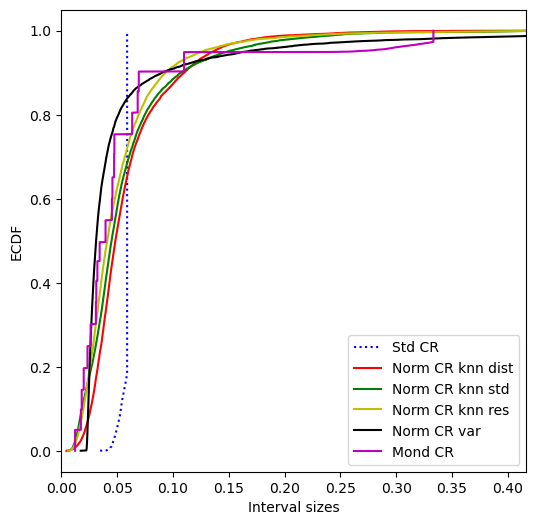
Let us look at the distribution of the interval sizes.
[77]:
interval_sizes = {}
for name in prediction_intervals.keys():
    interval_sizes[name] = prediction_intervals[name][:,1] \
    - prediction_intervals[name][:,0]

plt.figure(figsize=(6,6))
plt.ylabel("ECDF")
plt.xlabel("Interval sizes")
plt.xlim(0,interval_sizes["Mond CR"].max()*1.25)

colors = ["b","r","g","y","k","m","c","orange"]

for i, name in enumerate(interval_sizes.keys()):
    if "Std" in name:
        style = "dotted"
    else:
        style = "solid"
    plt.plot(np.sort(interval_sizes[name]),
             [i/len(interval_sizes[name])
              for i in range(1,len(interval_sizes[name])+1)],
             linestyle=style, c=colors[i], label=name)

plt.legend()
plt.show()
Evaluating the conformal regressors#
Let us put the six above conformal regressors in a dictionary:
[78]:
all_methods = {
    "Std CR": rf,
    "Norm CR knn dist": rf_norm_knn_dist,
    "Norm CR knn std": rf_norm_knn_std,
    "Norm CR knn res": rf_norm_knn_res,
    "Norm CR var" : rf_norm_var,
    "Mond CR": rf_mond
}
Let us evaluate them using three confidence levels on the test set. We could specify a subset of the metrics to use by the named metrics argument of the evaluate method; here we use all, which is the default.
[79]:
confidence_levels = [0.9,0.95,0.99]

names = list(all_methods.keys())

all_results = {}

for confidence in confidence_levels:
    for name in names:
        all_results[(name,confidence)] = all_methods[name].evaluate(
            X_test, y=y_test, confidence=confidence,
            y_min=0, y_max=1)

results_df = pd.DataFrame(columns=pd.MultiIndex.from_product(
    [names,confidence_levels]), index=list(list(
    all_results.values())[0].keys()))

for key in all_results.keys():
    results_df[key] = all_results[key].values()

display(results_df.round(4))
| Std CR | Norm CR knn dist | Norm CR knn std | Norm CR knn res | Norm CR var | Mond CR | |||||||||||||
|---|---|---|---|---|---|---|---|---|---|---|---|---|---|---|---|---|---|---|
| 0.90 | 0.95 | 0.99 | 0.90 | 0.95 | 0.99 | 0.90 | 0.95 | 0.99 | 0.90 | 0.95 | 0.99 | 0.90 | 0.95 | 0.99 | 0.90 | 0.95 | 0.99 | |
| error | 0.0982 | 0.0505 | 0.0102 | 0.1008 | 0.0482 | 0.0108 | 0.1022 | 0.0505 | 0.0101 | 0.1006 | 0.0519 | 0.0093 | 0.1030 | 0.0536 | 0.0093 | 0.1014 | 0.0512 | 0.0079 |
| eff_mean | 0.0420 | 0.0596 | 0.1248 | 0.0443 | 0.0594 | 0.0922 | 0.0438 | 0.0576 | 0.0917 | 0.0410 | 0.0541 | 0.0890 | 0.0448 | 0.0557 | 0.0824 | 0.0402 | 0.0520 | 0.0875 |
| eff_med | 0.0422 | 0.0613 | 0.1250 | 0.0357 | 0.0483 | 0.0756 | 0.0341 | 0.0451 | 0.0728 | 0.0320 | 0.0424 | 0.0700 | 0.0251 | 0.0317 | 0.0493 | 0.0272 | 0.0340 | 0.0582 |
| ks_test | 0.5216 | 0.5216 | 0.5216 | 0.5582 | 0.5582 | 0.5582 | 0.6790 | 0.6790 | 0.6790 | 0.6238 | 0.6238 | 0.6238 | 0.5837 | 0.5837 | 0.5837 | 0.5889 | 0.5889 | 0.5889 |
| time_fit | 0.0001 | 0.0001 | 0.0001 | 0.0001 | 0.0001 | 0.0001 | 0.0001 | 0.0001 | 0.0001 | 0.0001 | 0.0001 | 0.0001 | 0.0000 | 0.0000 | 0.0000 | 0.0002 | 0.0002 | 0.0002 |
| time_evaluate | 0.1550 | 0.1844 | 0.1336 | 0.2255 | 0.1752 | 0.1744 | 0.1511 | 0.1470 | 0.1698 | 0.1749 | 0.2008 | 0.1738 | 0.1579 | 0.1318 | 0.1306 | 0.0813 | 0.0753 | 0.0806 |
Semi-online conformal regressors#
Similar to semi-online conformal classifiers, we may consider employing online calibration also for conformal regressors, i.e., continuously updating the calibration set after making each prediction. This is achieved by setting online=True when calling the methods predict_p, predict_int and evaluate.
Online calibration with calibrated conformal regressors#
Here we will obtain p-values computed in an online fashion for some of the above calibrated conformal regressors. Note that in addition to the test objects, we also need to provide the correct labels.
[80]:
p_values = rf.predict_p(X_test, y_test, online=True)

display(p_values)

plt.ecdf(p_values)
plt.xlim(0,1)
plt.xlabel("p-value")
plt.ylabel("ECDF")
plt.show()

print(f"KS-test: {kstest(p_values, "uniform").pvalue}")
array([0.52848618, 0.06627263, 0.17079458, ..., 0.08839887, 0.23576108,
       0.72739162])

KS-test: 0.5156618639322833
[81]:
p_values = rf_norm_knn_dist.predict_p(X_test, y_test, online=True)

display(p_values)

plt.ecdf(p_values)
plt.xlim(0,1)
plt.xlabel("p-value")
plt.ylabel("ECDF")
plt.show()

print(f"KS-test: {kstest(p_values, "uniform").pvalue}")
array([0.29524717, 0.03850906, 0.17772657, ..., 0.29814802, 0.10931953,
       0.77414374])

KS-test: 0.5409239510089872
[82]:
p_values = rf_mond.predict_p(X_test, y_test, online=True)

display(p_values)

plt.ecdf(p_values)
plt.xlim(0,1)
plt.xlabel("p-value")
plt.ylabel("ECDF")
plt.show()

print(f"KS-test: {kstest(p_values, "uniform").pvalue}")
array([0.31872544, 0.02449724, 0.21532819, ..., 0.64472657, 0.04185852,
       0.82027838])

KS-test: 0.3834671667004743
Similarly, we can obtain prediction intervals using online calibration:
[83]:
rf.predict_int(X_test, y_test, online=True)
[83]:
array([[-0.00541253,  0.05344703],
       [ 0.03720586,  0.09606542],
       [ 0.03566307,  0.09452263],
       ...,
       [ 0.15016932,  0.21113679],
       [-0.01063683,  0.05033064],
       [ 0.04712939,  0.10809686]])
[84]:
rf_norm_knn_dist.predict_int(X_test, y_test, online=True)
[84]:
array([[0.01097246, 0.03706205],
       [0.04218894, 0.09108234],
       [0.03781259, 0.09237312],
       ...,
       [0.11997394, 0.24133216],
       [0.00370374, 0.03599006],
       [0.04805605, 0.10717021]])
[85]:
rf_mond.predict_int(X_test, y_test, online=True)
[85]:
array([[0.0140252 , 0.03400931],
       [0.04378119, 0.08949009],
       [0.04115257, 0.08903314],
       ...,
       [0.05815101, 0.3031551 ],
       [0.00914311, 0.03055069],
       [0.05163556, 0.1035907 ]])
By default, the test objects and labels are sequentially added to the existing calibration set, i.e., the one used when fitting the conformal regressor. We may set the warm_start option to False, if we would like to ignore the original calibration set. Note that the initial predictions tend to be very (maximally) wide, before we have a sufficiently large calibration set to allow for providing tighter intervals at the specified level of confidence.
[86]:
rf.predict_int(X_test, y_test, confidence=0.99, y_min=0, y_max=1,
               online=True, warm_start=False)
[86]:
array([[0.        , 1.        ],
       [0.        , 1.        ],
       [0.        , 1.        ],
       ...,
       [0.10530689, 0.25599921],
       [0.        , 0.09519306],
       [0.00226697, 0.15295929]])
[87]:
rf_norm_knn_dist.predict_int(X_test, y_test, confidence=0.99,
                             y_min=0, y_max=1,
                             online=True, warm_start=False)
[87]:
array([[0.        , 1.        ],
       [0.        , 1.        ],
       [0.        , 1.        ],
       ...,
       [0.07614989, 0.28515622],
       [0.        , 0.04764908],
       [0.02670914, 0.12851711]])
[88]:
rf_mond.predict_int(X_test, y_test, confidence=0.99,
                    y_min=0, y_max=1,
                    online=True, warm_start=False)
[88]:
array([[0.        , 1.        ],
       [0.        , 1.        ],
       [0.        , 1.        ],
       ...,
       [0.        , 0.38436009],
       [0.00262396, 0.03706984],
       [0.03225688, 0.12296937]])
We may also evaluate the conformal regressors using online calibration, by specifying online=True for the evaluate method:
[89]:
rf.evaluate(X_test, y_test, confidence=0.99, y_min=0, y_max=1, online=True)
[89]:
{'error': 0.010178587952253126,
 'eff_mean': 0.12478561796805053,
 'eff_med': 0.12495457547541068,
 'ks_test': 0.5216238604624142,
 'time_fit': 9.918212890625e-05,
 'time_evaluate': 0.13918805122375488}
[90]:
rf_norm_knn_dist.evaluate(X_test, y_test, confidence=0.99, y_min=0, y_max=1,
                          online=True)
[90]:
{'error': 0.010826316276487447,
 'eff_mean': 0.0922428113157142,
 'eff_med': 0.07555457247250805,
 'ks_test': 0.558158889497741,
 'time_fit': 7.081031799316406e-05,
 'time_evaluate': 0.17260098457336426}
[91]:
rf_mond.evaluate(X_test, y_test, confidence=0.99, y_min=0, y_max=1,
                 online=True)
[91]:
{'error': 0.007865272508559285,
 'eff_mean': 0.08751324207895611,
 'eff_med': 0.05817462399999982,
 'ks_test': 0.5888980645881281,
 'time_fit': 0.00020384788513183594,
 'time_evaluate': 0.07385849952697754}
Again, we may consider ignoring the original calibration set by setting warm_start=False:
[92]:
rf_norm_knn_dist.evaluate(X_test, y_test, confidence=0.99, y_min=0, y_max=1,
                          online=True, warm_start=False)
[92]:
{'error': 0.010271120570000902,
 'eff_mean': 0.09256447367994558,
 'eff_med': 0.0758803786845727,
 'ks_test': 0.0004459206100578574,
 'time_fit': 7.081031799316406e-05,
 'time_evaluate': 0.10671520233154297}
Online calibration without an initial calibration set#
Since the calibration set is incrementally extended during online calibration, we may consider starting with an empty calibration set; this allows us to use the full training set when fitting the underlying model.
[93]:
rf_full = WrapRegressor(RandomForestRegressor(n_jobs=-1, n_estimators=500,
                                              oob_score=True))

rf_full.fit(X_train, y_train)
Let us first initialize the conformal regressor with an empty calibration set, i.e., not specifying any objects or labels for the calibrate method (as we will see further below, we may still provide other parameters such as difficulty estimator, Mondrian categorizer, etc.):
[94]:
rf_full.calibrate()
[94]:
WrapRegressor(learner=RandomForestRegressor(n_estimators=500, n_jobs=-1, oob_score=True), calibrated=False)
We may now obtain prediction intervals while sequentially updating the calibration set:
[95]:
rf_full.predict_int(X_test, y_test, confidence=0.9, online=True)
[95]:
array([[       -inf,         inf],
       [       -inf,         inf],
       [       -inf,         inf],
       ...,
       [ 0.15874523,  0.1992304 ],
       [-0.00029073,  0.04021435],
       [ 0.05630021,  0.09680529]])
If we provide also a difficulty estimator to calibrate, we will obtain a normalized conformal regressor:
[96]:
de_var = DifficultyEstimator()
de_var.fit(X=X_train, learner=rf_full.learner, scaler=True)

rf_full.calibrate(de=de_var)
[96]:
WrapRegressor(learner=RandomForestRegressor(n_estimators=500, n_jobs=-1, oob_score=True), calibrated=False)
Now we get the intervals in the usual way:
[97]:
rf_full.predict_int(X_test, y_test, confidence=0.9, online=True)
[97]:
array([[      -inf,        inf],
       [      -inf,        inf],
       [      -inf,        inf],
       ...,
       [0.10515189, 0.25282374],
       [0.00556816, 0.03435545],
       [0.06027779, 0.09282772]])
We get a Mondrian regressor by providing a Mondrian categorizer to calibrate:
[98]:
mc = MondrianCategorizer()
mc.fit(X_cal, de=de_var, no_bins=10)

rf_full.calibrate(mc=mc)
[98]:
WrapRegressor(learner=RandomForestRegressor(n_estimators=500, n_jobs=-1, oob_score=True), calibrated=False)
We use the same call again to get the intervals from the Mondrian regressor:
[99]:
rf_full.predict_int(X_test, y_test, confidence=0.9, online=True)
[99]:
array([[      -inf,        inf],
       [      -inf,        inf],
       [      -inf,        inf],
       ...,
       [0.1265039 , 0.23147174],
       [0.01093225, 0.02899136],
       [0.05495483, 0.09815068]])
Let us investigate the coverage and prediction interval size for each category (here limiting the lower and upper bounds of the intervals):
[100]:
prediction_intervals = rf_full.predict_int(X_test, y_test, y_min=0,
                                           y_max=1, confidence=0.9, online=True)
number = []
coverage = []
size = []

bins_test = mc.apply(X_test)

for c in range(len(mc.bin_thresholds)-1):
    selection = bins_test == c
    number.append(np.sum(selection))
    coverage.append(np.sum(
        (prediction_intervals[selection,0] <= y_test[selection]) & \
        (y_test[selection] <= prediction_intervals[selection,1]))/np.sum(selection))
    size.append(np.sum(prediction_intervals[selection,1]-\
                       prediction_intervals[selection,0])/np.sum(selection))

df = pd.DataFrame({"Number":number, "Coverage":coverage, "Size":size})
df.round(4)
[100]:
| Number | Coverage | Size | |
|---|---|---|---|
| 0 | 147 | 0.8980 | 0.0799 |
| 1 | 506 | 0.9150 | 0.0319 |
| 2 | 602 | 0.8937 | 0.0291 |
| 3 | 736 | 0.9090 | 0.0309 |
| 4 | 965 | 0.9067 | 0.0288 |
| 5 | 1064 | 0.9004 | 0.0308 |
| 6 | 1275 | 0.8933 | 0.0326 |
| 7 | 1698 | 0.9028 | 0.0373 |
| 8 | 2003 | 0.9016 | 0.0482 |
| 9 | 1811 | 0.9061 | 0.1129 |
Let us investigate also the p-values:
[101]:
p_values = rf_full.predict_p(X_test, y_test, online=True)

display(p_values)

plt.ecdf(p_values)
plt.xlim(0,1)
plt.xlabel("p-value")
plt.ylabel("ECDF")
plt.show()

print(f"KS-test: {kstest(p_values, "uniform").pvalue}")
array([0.20102592, 0.38311158, 0.7211436 , ..., 0.38319377, 0.04702385,
       0.76717759])
KS-test: 0.6739330554339684
We may also evaluate the conformal regressor using online calibration, by specifying online=True for the evaluate method:
[102]:
rf_full.evaluate(X_test, y_test, confidence=0.99, y_min=0, y_max=1, online=True)
[102]:
{'error': 0.008235402979550277,
 'eff_mean': 0.17126926926893468,
 'eff_med': 0.06663963304918027,
 'ks_test': 0.12346439081948901,
 'time_fit': 1.0251998901367188e-05,
 'time_evaluate': 0.08956360816955566}
Out-of-bag calibration#
For conformal regressors that employ learners that use bagging, like random forests, we may consider an alternative strategy to dividing the original training set into a proper training and calibration set; we may use the out-of-bag (OOB) predictions, which allow us to use the full training set for both model building and calibration. It should be noted that this strategy does not come with the theoretical validity guarantee of the above (inductive) conformal regressors, due to that calibration and test instances are not handled in exactly the same way. In practice, however, conformal regressors based on out-of-bag predictions rarely fail to meet the coverage requirements.
Standard conformal regressors with out-of-bag calibration#
Let us first generate a model from the full training set, making sure the learner has an attribute oob_prediction_, which e.g. is the case for a RandomForestRegressor if oob_score is set to True when created.
[103]:
learner_full = RandomForestRegressor(n_jobs=-1, n_estimators=500, oob_score=True)

rf = WrapRegressor(learner_full)

rf.fit(X_train, y_train)
We may now obtain a standard conformal regressor using OOB predictions:
[104]:
rf.calibrate(X_train, y_train, oob=True)

display(rf)
WrapRegressor(learner=RandomForestRegressor(n_estimators=500, n_jobs=-1, oob_score=True), calibrated=True, predictor=ConformalRegressor(fitted=True, normalized=False, mondrian=False))
… and apply it using the point predictions of the full model.
[105]:
intervals_std_oob = rf.predict_int(X_test, y_min=0, y_max=1)

display(intervals_std_oob)
array([[0.        , 0.05392285],
       [0.03392021, 0.09471719],
       [0.03367333, 0.09447031],
       ...,
       [0.1512086 , 0.21200558],
       [0.        , 0.05081027],
       [0.04670459, 0.10750157]])
Normalized conformal regressors with out-of-bag calibration#
We may also generate normalized conformal regressors from the OOB predictions. The DifficultyEstimator can be used also for this purpose; for the k-nearest neighbor approaches, the difficulty of each object in the training set will be computed using a leave-one-out procedure, while for the variance-based approach the out-of-bag predictions will be employed.
By setting oob=True, we inform the fit method that we may request difficulty estimates for the provided set of objects; these will be retrieved by not providing any objects when calling the apply method.
Let us start with the k-nearest neighbor approach using distances only.
[106]:
de_knn_dist_oob = DifficultyEstimator()

de_knn_dist_oob.fit(X=X_train, scaler=True, oob=True)

display(de_knn_dist_oob)

rf.calibrate(X_train, y_train, de=de_knn_dist_oob, oob=True)

display(rf)
DifficultyEstimator(fitted=True, type=knn, k=25, target=none, scaler=True, beta=0.01, oob=True)
WrapRegressor(learner=RandomForestRegressor(n_estimators=500, n_jobs=-1, oob_score=True), calibrated=True, predictor=ConformalRegressor(fitted=True, normalized=True, mondrian=False))
We may then apply the normalized conformal OOB regressor to the test set, as usual:
[107]:
sigmas_test_knn_dist_oob = de_knn_dist_oob.apply(X_test)

intervals_norm_knn_dist_oob = rf.predict_int(X_test, y_min=0, y_max=1)

display(intervals_norm_knn_dist_oob)
array([[0.00899123, 0.03805748],
       [0.03611455, 0.09252284],
       [0.0327914 , 0.09535224],
       ...,
       [0.11675731, 0.24645686],
       [0.00288415, 0.03793941],
       [0.04528273, 0.10892344]])
For completeness, we will illustrate the use of out-of-bag calibration for the remaining approaches too. For k-nearest neighbors with labels, we do the following:
[108]:
de_knn_std_oob = DifficultyEstimator()

de_knn_std_oob.fit(X=X_train, y=y_train, scaler=True, oob=True)

display(de_knn_std_oob)

rf.calibrate(X_train, y_train, de=de_knn_std_oob, oob=True)

display(rf)

intervals_norm_knn_std_oob = rf.predict_int(X_test, y_min=0, y_max=1)

display(intervals_norm_knn_std_oob)
DifficultyEstimator(fitted=True, type=knn, k=25, target=labels, scaler=True, beta=0.01, oob=True)
WrapRegressor(learner=RandomForestRegressor(n_estimators=500, n_jobs=-1, oob_score=True), calibrated=True, predictor=ConformalRegressor(fitted=True, normalized=True, mondrian=False))
array([[0.01672016, 0.03032854],
       [0.03244135, 0.09619604],
       [0.04584447, 0.08229917],
       ...,
       [0.12225957, 0.2409546 ],
       [0.0134443 , 0.02737926],
       [0.06053929, 0.09366687]])
A third option is to use k-nearest neighbors with (OOB) residuals:
[109]:
residuals_oob = y_train - learner_full.oob_prediction_

de_knn_res_oob = DifficultyEstimator()

de_knn_res_oob.fit(X=X_train, residuals=residuals_oob, scaler=True, oob=True)

display(de_knn_res_oob)

rf.calibrate(X_train, y_train, de=de_knn_res_oob, oob=True)

display(rf)

intervals_norm_knn_res_oob = rf.predict_int(X_test, y_min=0, y_max=1)

display(intervals_norm_knn_res_oob)
DifficultyEstimator(fitted=True, type=knn, k=25, target=residuals, scaler=True, beta=0.01, oob=True)
WrapRegressor(learner=RandomForestRegressor(n_estimators=500, n_jobs=-1, oob_score=True), calibrated=True, predictor=ConformalRegressor(fitted=True, normalized=True, mondrian=False))
array([[0.01523718, 0.03181153],
       [0.0302243 , 0.09841309],
       [0.04152951, 0.08661412],
       ...,
       [0.14021296, 0.22300121],
       [0.0134985 , 0.02732505],
       [0.05715833, 0.09704784]])
A fourth and final option for the normalized conformal regressors is to use variance as a difficulty estimate. We then leave labels and residuals out, but provide an (ensemble) learner. In contrast to when oob=False, we are here required to provide the (full) training set, from which the variance of the out-of-bag predictions will be computed. When applied to the test set, the full ensemble model will not be used to obtain the difficulty estimates, but instead a subset of the constituent
models is used, following what could be seen as post hoc assignment of each test instance to a bag.
[110]:
de_var_oob = DifficultyEstimator()

de_var_oob.fit(X=X_train, learner=learner_full, scaler=True, oob=True)

display(de_var_oob)

rf.calibrate(X_train, y_train, de=de_var_oob, oob=True)

display(rf)

intervals_norm_var_oob = rf.predict_int(X_test, y_min=0, y_max=1)

display(intervals_norm_var_oob)
DifficultyEstimator(fitted=True, type=variance, scaler=True, beta=0.01, oob=True)
WrapRegressor(learner=RandomForestRegressor(n_estimators=500, n_jobs=-1, oob_score=True), calibrated=True, predictor=ConformalRegressor(fitted=True, normalized=True, mondrian=False))
array([[0.00414253, 0.04290618],
       [0.0418052 , 0.0868322 ],
       [0.0413419 , 0.08680174],
       ...,
       [0.08592402, 0.27729015],
       [0.00087813, 0.03994543],
       [0.05513471, 0.09907146]])
Mondrian conformal regressors with out-of-bag calibration#
We may form the categories using the difficulty estimator obtained from the OOB predictions. We here consider the difficulty estimates produced by the fourth above option (using variance) only.
[111]:
mc_oob = MondrianCategorizer()

mc_oob.fit(de=de_var_oob, oob=True, no_bins=20)

display(mc_oob)

rf.calibrate(X_train, y_train, mc=mc_oob, oob=True)

display(rf)
MondrianCategorizer(fitted=True, de=DifficultyEstimator(fitted=True, type=variance, scaler=True, beta=0.01, oob=True), no_bins=20)
WrapRegressor(learner=RandomForestRegressor(n_estimators=500, n_jobs=-1, oob_score=True), calibrated=True, predictor=ConformalRegressor(fitted=True, normalized=False, mondrian=True))
Let us generate prediction intervals:
[112]:
intervals_mond_oob = rf.predict_int(X_test, y_min=0, y_max=1)

display(intervals_mond_oob)
array([[0.01132043, 0.03572828],
       [0.03530293, 0.09333447],
       [0.03529444, 0.0928492 ],
       ...,
       [0.05935642, 0.30385775],
       [0.00785379, 0.03296977],
       [0.04808731, 0.10611885]])
Investigating the OOB prediction intervals#
[113]:
prediction_intervals = {
    "Std CR OOB":intervals_std_oob,
    "Norm CR knn dist OOB":intervals_norm_knn_dist_oob,
    "Norm CR knn std OOB":intervals_norm_knn_std_oob,
    "Norm CR knn res OOB":intervals_norm_knn_res_oob,
    "Norm CR var OOB":intervals_norm_var_oob,
    "Mond CR OOB":intervals_mond_oob,
}
Let us see what fraction of the intervals that contain the true targets and how large the intervals are.
[114]:
coverages = []
mean_sizes = []
median_sizes = []

for name in prediction_intervals.keys():
    intervals = prediction_intervals[name]
    coverages.append(np.sum([1 if (y_test[i]>=intervals[i,0] and
                                   y_test[i]<=intervals[i,1]) else 0
                            for i in range(len(y_test))])/len(y_test))
    mean_sizes.append((intervals[:,1]-intervals[:,0]).mean())
    median_sizes.append(np.median((intervals[:,1]-intervals[:,0])))

pred_int_df = pd.DataFrame({"Coverage":coverages,
                            "Mean size":mean_sizes,
                            "Median size":median_sizes},
                           index=list(prediction_intervals.keys()))

pred_int_df.loc["Mean"] = [pred_int_df["Coverage"].mean(),
                           pred_int_df["Mean size"].mean(),
                           pred_int_df["Median size"].mean()]

display(pred_int_df.round(4))
| Coverage | Mean size | Median size | |
|---|---|---|---|
| Std CR OOB | 0.9501 | 0.0594 | 0.0608 |
| Norm CR knn dist OOB | 0.9663 | 0.0656 | 0.0538 |
| Norm CR knn std OOB | 0.9502 | 0.0561 | 0.0441 |
| Norm CR knn res OOB | 0.9360 | 0.0488 | 0.0382 |
| Norm CR var OOB | 0.9531 | 0.0500 | 0.0406 |
| Mond CR OOB | 0.9525 | 0.0514 | 0.0387 |
| Mean | 0.9514 | 0.0552 | 0.0460 |
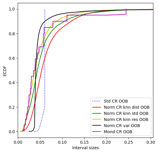
Let us look at the distribution of the interval sizes.
[115]:
interval_sizes = {}
for name in prediction_intervals.keys():
    interval_sizes[name] = prediction_intervals[name][:,1] \
    - prediction_intervals[name][:,0]

plt.figure(figsize=(6,6))
plt.ylabel("ECDF")
plt.xlabel("Interval sizes")
plt.xlim(0,interval_sizes["Mond CR OOB"].max()*1.25)

colors = ["b","r","g","y","k","m","c","orange"]

for i, name in enumerate(interval_sizes.keys()):
    if "Std" in name:
        style = "dotted"
    else:
        style = "solid"
    plt.plot(np.sort(interval_sizes[name]),
             [i/len(interval_sizes[name])
              for i in range(1,len(interval_sizes[name])+1)],
             linestyle=style, c=colors[i], label=name)

plt.legend()
plt.show()
Conformal predictive systems#
Creating and fitting conformal predictive systems#
Conformal predictive systems are created through the WrapRegressor class in the same way as conformal regressors. We specify that a conformal predictive system, rather than a conformal regressor, should be formed by providing cps=True when calling the calibrate method (default is cps=False).
Let us start by generating standard and normalized conformal predictive systems (CPS), using the previously fitted learner_prop and difficulty estimator de_var, as well two conformal predictive systems relying on out-of-bag predictions, using the previously fitted learner_full with and without normalization, in the former case using the difficulty estimator de_var_oob.
[116]:
cps_std = WrapRegressor(learner_prop)

cps_std.calibrate(X_cal, y_cal, cps=True)

display(cps_std)

cps_norm = WrapRegressor(learner_prop).calibrate(X_cal, y_cal, de=de_knn_std,
                                                 cps=True)
display(cps_norm)

cps_std_oob = WrapRegressor(learner_full).calibrate(X_train, y_train, oob=True,
                                                    cps=True)
display(cps_std_oob)

cps_norm_oob = WrapRegressor(learner_full).calibrate(X_train, y_train,
                                                     de=de_var_oob, oob=True, cps=True)
display(cps_norm_oob)
WrapRegressor(learner=RandomForestRegressor(n_estimators=500, n_jobs=-1, oob_score=True), calibrated=True, predictor=ConformalPredictiveSystem(fitted=True, normalized=False, mondrian=False))
WrapRegressor(learner=RandomForestRegressor(n_estimators=500, n_jobs=-1, oob_score=True), calibrated=True, predictor=ConformalPredictiveSystem(fitted=True, normalized=True, mondrian=False))
Let us also create some Mondrian CPS, but in contrast to the Mondrian conformal regressors above, we here form the categories through binning of the predictions rather than binning of the difficulty estimates. We also show how we still may use the latter to obtain a normalized CPS for each category (bin).
[117]:
mc_p = MondrianCategorizer()

mc_p.fit(X_cal, f=learner_prop.predict, no_bins=5)

cps_mond_std = WrapRegressor(learner_prop)
cps_mond_std.calibrate(X_cal, y_cal, mc=mc_p, cps=True)

display(cps_mond_std)

cps_mond_norm = WrapRegressor(learner_prop)
cps_mond_norm.calibrate(X_cal, y_cal, de=de_knn_std, mc=mc_p, cps=True)

display(cps_mond_norm)

mc_p_oob = MondrianCategorizer()
mc_p_oob.fit(learner=learner_full, oob=True, no_bins=5)

display(mc_p_oob)

cps_mond_std_oob = WrapRegressor(learner_full)
cps_mond_std_oob.calibrate(X_train, y_train, mc=mc_p_oob, oob=True, cps=True)

display(cps_mond_std_oob)

cps_mond_norm_oob = WrapRegressor(learner_full)
cps_mond_norm_oob.calibrate(X_train, y_train, de=de_var_oob, mc=mc_p_oob, oob=True, cps=True)

display(cps_mond_norm_oob)
WrapRegressor(learner=RandomForestRegressor(n_estimators=500, n_jobs=-1, oob_score=True), calibrated=True, predictor=ConformalPredictiveSystem(fitted=True, normalized=False, mondrian=True))
WrapRegressor(learner=RandomForestRegressor(n_estimators=500, n_jobs=-1, oob_score=True), calibrated=True, predictor=ConformalPredictiveSystem(fitted=True, normalized=True, mondrian=True))
MondrianCategorizer(fitted=True, learner=RandomForestRegressor(n_estimators=500, n_jobs=-1, oob_score=True), no_bins=5)
WrapRegressor(learner=RandomForestRegressor(n_estimators=500, n_jobs=-1, oob_score=True), calibrated=True, predictor=ConformalPredictiveSystem(fitted=True, normalized=False, mondrian=True))
WrapRegressor(learner=RandomForestRegressor(n_estimators=500, n_jobs=-1, oob_score=True), calibrated=True, predictor=ConformalPredictiveSystem(fitted=True, normalized=True, mondrian=True))
Making predictions#
We still have access to the usual predict method, to obtain point predictions of the wrapped learner, as well as the predict_p and predict_int methods, which work as for conformal regressors. There are also some methods that are specific to conformal predictive systems; predict_percentiles and predict_cpds that are used for obtaining percentiles and conformal predictive distributions, respectively. In addition, there is also a method called predict_cps, for which the
output will depend on how we specify the input and which can be used for getting all of the above by just one method call.
Here we will obtain the p-values from cps_mond_norm for the true targets of the test set:
[118]:
p_values = cps_mond_norm.predict_p(X_test, y_test, seed=123)

display(p_values)
array([0.17471673, 0.06707235, 0.06696276, ..., 0.20351712, 0.00770605,
       0.65840421])
Let us take a look at how the p-values are distributed. From the visual inspection they may appear be approximaly uniformly distributed; this is however not guaranteed, since the p-values are not independent (see further below for semi-online conformal predictive systems, for which this indeed holds). It is hence not very surprising if the Kolmogorov-Smirnov test allows us to reject that the p-values are sampled from a uniform distribution.
[119]:
plt.ecdf(p_values)
plt.xlim(0,1)
plt.xlabel("p-value")
plt.ylabel("ECDF")
plt.show()

print(f"KS-test: {kstest(p_values, "uniform").pvalue}")
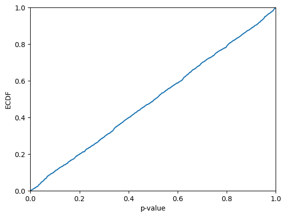
KS-test: 0.005174753868863953
We can get the same result through predict_cps in the following way:
[120]:
p_values = cps_mond_norm.predict_cps(X_test, y=y_test, seed=123)

display(p_values)
array([0.17471673, 0.06707235, 0.06696276, ..., 0.20351712, 0.00770605,
       0.65840421])
If we instead would like to get threshold values, such that the probability for the true target is less than the threshold for each test instance, we may request these through predict_percentiles or by providing lower_percentiles and/or upper_percentiles as input to the predict_cps method. These denote (one or more) percentiles for which a lower (upper) value will be selected in case a percentile lies between two values (similar to interpolation="lower" and
interpolation="higher" in numpy.percentile).
Here we will obtain the lowest values from cps_mond_norm, such that the probability for the target values being less than these is at least 50%, first using predict_percentiles:
[121]:
thresholds = cps_mond_norm.predict_percentiles(X_test, higher_percentiles=50)

display(thresholds)
array([0.02385006, 0.06575971, 0.06462498, ..., 0.17986191, 0.01973645,
       0.07719558])
Again, the same result can be obtained using the predict_cps method:
[122]:
thresholds = cps_mond_norm.predict_cps(X_test, higher_percentiles=50)

display(thresholds)
array([0.02385006, 0.06575971, 0.06462498, ..., 0.17986191, 0.01973645,
       0.07719558])
For the predict_cps method, we can also specify both target values and percentiles; the resulting p-values will be returned in the first column, while any values corresponding to the lower percentiles will be included in the subsequent columns, followed by columns containing the values corresponding to the higher percentiles. The following call hence results in an array with five columns:
[123]:
results = cps_mond_norm.predict_cps(X_test, y=y_test,
                                    lower_percentiles=[2.5, 5],
                                    higher_percentiles=[95, 97.5])

display(results)
array([[0.17434064, 0.01149596, 0.01503237, 0.03121168, 0.03400184],
       [0.0676628 , 0.02888577, 0.03805115, 0.09196404, 0.09760103],
       [0.06705096, 0.04492915, 0.04982474, 0.07862176, 0.08163269],
       ...,
       [0.20299627, 0.11379486, 0.13265114, 0.24114184, 0.25741495],
       [0.00844923, 0.01157506, 0.01391129, 0.0245997 , 0.02644294],
       [0.65934984, 0.05961798, 0.06398707, 0.08968703, 0.09237415]])
In addition to p-values and threshold values, we can request that the conformal predictive system returns the full conformal predictive distribution (CPD) for each test instance, as defined by the threshold values, either by the predict_cpds method or by setting return_cpds=True for the predict_cps method . The format of the distributions vary with the type of conformal predictive system; for a standard and normalized CPS, the output is an array with a row for each test instance and
a column for each calibration instance (residual), while for a Mondrian CPS, the default output is a vector containing one CPD per test instance (since the number of values may vary between categories). If the desired output instead is an array of distributions per category, where all distributions in a category have the same number of columns, which in turn depends on the number of calibration instances in the corresponding category, then cpds_by_bins=True may be specified (for both
methods). In case return_cpds=True is specified together with y, lower_percentiles or higher_percentiles, the output of predict will be a pair, with the first element holding the results of the above type and the second element will contain the CPDs.
For the above Mondrian CPS, the following call to predict_cpds will result in a vector of distributions, with one element for each test instance.
[124]:
cpds = cps_mond_norm.predict_cpds(X_test)

print(f"No. of test instances: {len(X_test)}")
print(f"Shape of cpds: {cpds.shape}")
No. of test instances: 10807
Shape of cpds: (10807,)
The same result can be obtained with the following call to predict_cps:
[125]:
cpds = cps_mond_norm.predict_cps(X_test, return_cpds=True)

print(f"No. of test instances: {len(X_test)}")
print(f"Shape of cpds: {cpds.shape}")
No. of test instances: 10807
Shape of cpds: (10807,)
If we instead would prefer to represent these distributions by one array per category, we set cpds_by_bins=True, noting that it will be a bit trickier to associate a test instance to a specific distribution.
[126]:
cpds = cps_mond_norm.predict_cps(X_test, return_cpds=True, cpds_by_bins=True)

for i, cpd in enumerate(cpds):
    print(f"bin {i}: {cpd.shape[0]} test instances, {cpd.shape[1]} threshold values")

print(f"No. of test instances: {sum([c.shape[0] for c in cpds])}")
bin 0: 2030 test instances, 541 threshold values
bin 1: 2258 test instances, 540 threshold values
bin 2: 2174 test instances, 540 threshold values
bin 3: 2178 test instances, 540 threshold values
bin 4: 2167 test instances, 541 threshold values
No. of test instances: 10807
We may also plot the conformal predictive distribution for some test object. In case the calibration set is very large, you may consider plotting an approximation of the full distribution by using a grid of values for lower_percentiles or higher_percentiles, instead of setting return_cpds=True. For the Mondrian CPS, the size of the calibration set for each bin is reasonable in this case, so we may just use the distributions directly.
[127]:
cpds = cps_mond_norm_oob.predict_cps(X_test, return_cpds=True)

test_index = np.random.randint(len(X_test)) # A test object is randomly selected
cpd = cpds[test_index]

p = np.array([i/len(cpd) for i in range(len(cpd))])

lower_index = np.where(p<=0.025)[0][-1]
mid_index = np.where(p>=0.50)[0][0]
upper_index = np.where(p>=0.975)[0][0]

low_percentile = cpd[lower_index]
median = cpd[mid_index]
high_percentile = cpd[upper_index]

plt.figure(figsize=(6,6))

y_hat = cps_mond_norm_oob.predict(X_test[test_index][None,:])

plt.plot([y_hat,y_hat],[0,1], color="tab:orange")
plt.plot([y_test[test_index],y_test[test_index]],[0,1], color="tab:red")
plt.xlabel("y")
plt.ylabel("Q(y)")
plt.ylim(0,1)

plt.plot([median,median],[0,1],"g--")
plt.plot([low_percentile,low_percentile],[0,1],"y--")
plt.legend(["ŷ","target","$y_{0.5}$","[$y_{0.025}$,$y_{0.975}$]"])
plt.plot([high_percentile,high_percentile],[0,1],"y--")
plt.plot(cpd,p, color="tab:blue")
rectangle = plt.Rectangle((low_percentile,0),
                          abs(high_percentile-low_percentile),1, color="y",
                          alpha=0.05)
plt.gca().add_patch(rectangle)
plt.show()
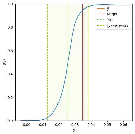
Investigating the coverage and size of extracted prediction intervals#
Let us investigate the extracted prediction intervals at the 95% confidence level. This is done by a specifying percentiles corresponding to the interval endpoints.
[128]:
all_cps = {"Std CPS":cps_std,
           "Std OOB CPS":cps_std_oob,
           "Norm CPS":cps_norm,
           "Norm OOB CPS":cps_norm_oob,
           "Mond CPS":cps_mond_std,
           "Mond OOB CPS":cps_mond_std_oob,
           "Mond norm CPS":cps_mond_norm,
           "Mond norm OOB CPS":cps_mond_norm_oob
          }

all_cps_intervals = {}

coverages = []
mean_sizes = []
median_sizes = []

for name in all_cps.keys():
    intervals = all_cps[name].predict_int(X_test, y_min=0, y_max=1)
    all_cps_intervals[name] = intervals
    coverages.append(np.sum([1 if (y_test[i]>=intervals[i,0] and
                                   y_test[i]<=intervals[i,1]) else 0
                            for i in range(len(y_test))])/len(y_test))
    mean_sizes.append((intervals[:,1]-intervals[:,0]).mean())
    median_sizes.append(np.median((intervals[:,1]-intervals[:,0])))

pred_int_df = pd.DataFrame({"Coverage":coverages,
                            "Mean size":mean_sizes,
                            "Median size":median_sizes},
                           index=list(all_cps_intervals.keys()))

pred_int_df.loc["Mean"] = [pred_int_df["Coverage"].mean(),
                           pred_int_df["Mean size"].mean(),
                           pred_int_df["Median size"].mean()]

display(pred_int_df.round(4))
| Coverage | Mean size | Median size | |
|---|---|---|---|
| Std CPS | 0.9463 | 0.0593 | 0.0603 |
| Std OOB CPS | 0.9498 | 0.0604 | 0.0614 |
| Norm CPS | 0.9516 | 0.0579 | 0.0454 |
| Norm OOB CPS | 0.9533 | 0.0512 | 0.0414 |
| Mond CPS | 0.9495 | 0.0588 | 0.0432 |
| Mond OOB CPS | 0.9503 | 0.0564 | 0.0415 |
| Mond norm CPS | 0.9491 | 0.0586 | 0.0416 |
| Mond norm OOB CPS | 0.9508 | 0.0520 | 0.0391 |
| Mean | 0.9501 | 0.0568 | 0.0468 |
Investigating the distributions of extracted prediction intervals#
Let us take a look at the distribution of the interval sizes.
[129]:
cps_interval_sizes = {}

for name in all_cps_intervals.keys():
    cps_interval_sizes[name] = \
    all_cps_intervals[name][:,1] - all_cps_intervals[name][:,0]

plt.figure(figsize=(6,6))
plt.ylabel("ECDF")
plt.xlabel("Interval sizes")
plt.xlim(0,cps_interval_sizes["Mond OOB CPS"].max()*1.25)

colors = ["b","r","g","y","k","m", "gray", "orange"]

for i, name in enumerate(cps_interval_sizes.keys()):
    if "Std" in name:
        style = "dotted"
    else:
        style = "solid"
    plt.plot(np.sort(cps_interval_sizes[name]),
             [i/len(cps_interval_sizes[name])
              for i in range(1,len(cps_interval_sizes[name])+1)],
             linestyle=style, c=colors[i], label=name)

plt.legend()
plt.show()
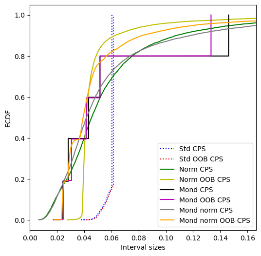
Extracting medians#
Let us take a look at the medians; they can be derived using either lower or higher interpolation, but ideally the differences should be small.
[130]:
all_cps_medians = {}

for name in all_cps.keys():
    medians = all_cps[name].predict_cps(X_test,
                                        lower_percentiles=50,
                                        higher_percentiles=50)
    all_cps_medians[name] = medians
    print(name)
    print("\tMean difference of the medians:    {:.6f}".format((medians[:,1]-medians[:,0]).mean()))
    print("\tLargest difference of the medians: {:.6f}".format((medians[:,1]-medians[:,0]).max()))
Std CPS
        Mean difference of the medians:    0.000006
        Largest difference of the medians: 0.000006
Std OOB CPS
        Mean difference of the medians:    0.000002
        Largest difference of the medians: 0.000002
Norm CPS
        Mean difference of the medians:    0.000007
        Largest difference of the medians: 0.000062
Norm OOB CPS
        Mean difference of the medians:    0.000001
        Largest difference of the medians: 0.000034
Mond CPS
        Mean difference of the medians:    0.000017
        Largest difference of the medians: 0.000046
Mond OOB CPS
        Mean difference of the medians:    0.000002
        Largest difference of the medians: 0.000005
Mond norm CPS
        Mean difference of the medians:    0.000027
        Largest difference of the medians: 0.000525
Mond norm OOB CPS
        Mean difference of the medians:    0.000005
        Largest difference of the medians: 0.000468
Another view of the medians and prediction intervals#
[131]:
y_hat_test = learner_prop.predict(X_test)
y_hat_full = learner_full.predict(X_test)

plt.subplots(len(all_cps_intervals.keys())//2,2,figsize=(12,24))

sorted_prop_indexes = np.argsort(y_hat_test)

sorted_full_indexes = np.argsort(y_hat_full)

alpha=0.2

for i, name in enumerate(all_cps_intervals.keys()):

    plt.subplot(len(all_cps_intervals.keys())//2,2,i+1)
    if "OOB" in name:
        indexes = sorted_full_indexes
        y_hat_ = y_hat_full
    else:
        indexes = sorted_prop_indexes
        y_hat_ = y_hat_test

    plt.title(name)
    plt.plot(y_hat_[indexes], all_cps_intervals[name][indexes,0],
             color="r", alpha=alpha)
    plt.plot(y_hat_[indexes], all_cps_intervals[name][indexes,1],
             color="r", alpha=alpha)
    plt.scatter(y_hat_[indexes],y_test[indexes],
                color="b", marker="o", alpha=alpha)
    plt.scatter(y_hat_[indexes],y_hat_[indexes],
                color="y", marker=".", alpha=alpha)
    plt.xlabel("predicted")
    plt.ylabel("endpoints")

plt.show()
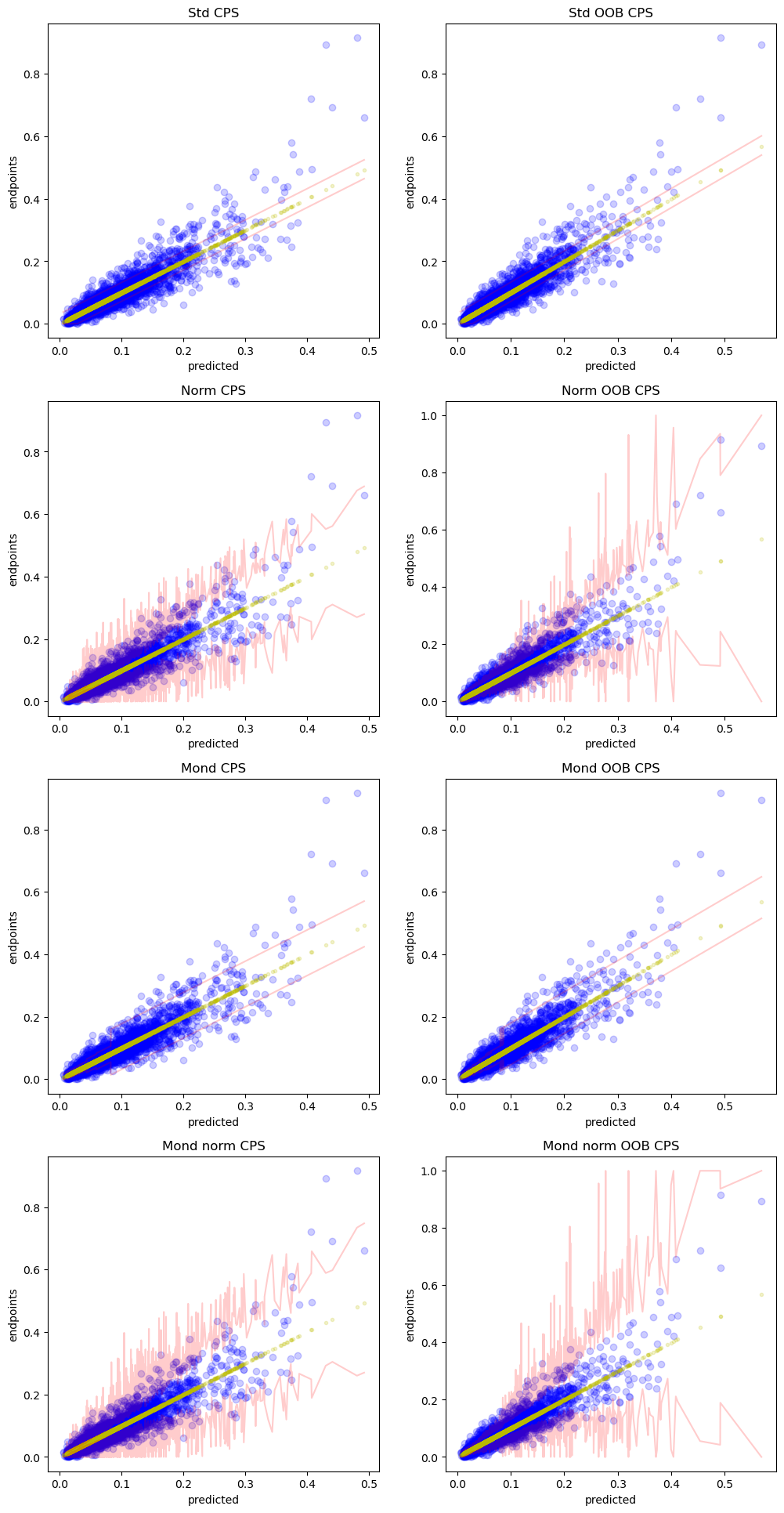
Evaluating the CPS using a test set#
Let us evaluate the generated CPS using three confidence levels on the test set. We could specify a subset of the metrics to use by the metrics parameter of the evaluate method; here we use all metrics, which is the default
Note that bins can always be provided, but they will be ignored by CPS that have not been fitted with such, i.e., the CPS is not of the Mondrian type.
Note that CRPS takes some time to compute, in particular when the CPS have been fitted with larger calibration sets.
[132]:
confidence_levels = [0.9,0.95,0.99]

names = np.array(list(all_cps.keys()))

first_set = names[["OOB" not in name for name in names]]
second_set = names[["OOB" in name for name in names]]

for methods in [first_set, second_set]:
    all_cps_results = {}
    for confidence in confidence_levels:
        for name in methods:
            all_cps_results[(name,confidence)] = all_cps[name].evaluate(
                    X_test, y=y_test, confidence=confidence,
                    y_min=0, y_max=1)

    cps_results_df = pd.DataFrame(columns=pd.MultiIndex.from_product(
        [methods,confidence_levels]), index=list(list(
        all_cps_results.values())[0].keys()))

    for key in all_cps_results.keys():
        cps_results_df[key] = all_cps_results[key].values()

    display(cps_results_df.round(4))
| Std CPS | Norm CPS | Mond CPS | Mond norm CPS | |||||||||
|---|---|---|---|---|---|---|---|---|---|---|---|---|
| 0.90 | 0.95 | 0.99 | 0.90 | 0.95 | 0.99 | 0.90 | 0.95 | 0.99 | 0.90 | 0.95 | 0.99 | |
| error | 0.0988 | 0.0512 | 0.0094 | 0.1021 | 0.0494 | 0.0101 | 0.1043 | 0.0499 | 0.0083 | 0.1036 | 0.0492 | 0.0098 |
| eff_mean | 0.0421 | 0.0609 | 0.1305 | 0.0438 | 0.0577 | 0.0920 | 0.0418 | 0.0594 | 0.1047 | 0.0451 | 0.0589 | 0.0961 |
| eff_med | 0.0423 | 0.0620 | 0.1333 | 0.0342 | 0.0452 | 0.0730 | 0.0292 | 0.0408 | 0.0727 | 0.0323 | 0.0424 | 0.0687 |
| time_fit | 0.0002 | 0.0002 | 0.0002 | 0.0000 | 0.0000 | 0.0000 | 0.0007 | 0.0007 | 0.0007 | 0.0006 | 0.0006 | 0.0006 |
| ks_test | 0.5863 | 0.5863 | 0.5863 | 0.5594 | 0.5594 | 0.5594 | 0.6178 | 0.6178 | 0.6178 | 0.6107 | 0.6107 | 0.6107 |
| time_evaluate | 0.1423 | 0.1394 | 0.1564 | 0.1394 | 0.1499 | 0.1305 | 0.0705 | 0.0779 | 0.0743 | 0.0973 | 0.0962 | 0.0806 |
| Std OOB CPS | Norm OOB CPS | Mond OOB CPS | Mond norm OOB CPS | |||||||||
|---|---|---|---|---|---|---|---|---|---|---|---|---|
| 0.90 | 0.95 | 0.99 | 0.90 | 0.95 | 0.99 | 0.90 | 0.95 | 0.99 | 0.90 | 0.95 | 0.99 | |
| error | 0.0970 | 0.0504 | 0.0110 | 0.0982 | 0.0475 | 0.0098 | 0.0991 | 0.0492 | 0.0089 | 0.0962 | 0.0480 | 0.0101 |
| eff_mean | 0.0416 | 0.0604 | 0.1247 | 0.0380 | 0.0508 | 0.0797 | 0.0419 | 0.0567 | 0.0965 | 0.0408 | 0.0518 | 0.0796 |
| eff_med | 0.0418 | 0.0614 | 0.1309 | 0.0307 | 0.0412 | 0.0652 | 0.0300 | 0.0397 | 0.0645 | 0.0290 | 0.0378 | 0.0604 |
| time_fit | 0.0003 | 0.0003 | 0.0003 | 0.0002 | 0.0002 | 0.0002 | 0.0003 | 0.0003 | 0.0003 | 0.0005 | 0.0005 | 0.0005 |
| ks_test | 0.4577 | 0.4577 | 0.4577 | 0.5029 | 0.5029 | 0.5029 | 0.3997 | 0.3997 | 0.3997 | 0.3922 | 0.3922 | 0.3922 |
| time_evaluate | 0.1687 | 0.1927 | 0.2239 | 0.1653 | 0.1574 | 0.1603 | 0.1169 | 0.0836 | 0.0823 | 0.1173 | 0.0946 | 0.1243 |
Semi-online conformal predictive systems#
Similar to semi-online conformal regressors and classifiers, we may consider employing online calibration also for conformal predictive systems, i.e., continuously updating the calibration set after making each prediction. This is achieved by setting online=True when calling the methods predict_p, predict_int, predict_percentiles, predict_cpds, and evaluate.
Online calibration with calibrated conformal predictive systems#
Here we will obtain p-values computed in an online fashion for some of the above calibrated conformal predictive systems. Note that in addition to the test objects, we also need to provide the correct labels.
[133]:
for cps in first_set:
    print(cps)
    p_values = all_cps[cps].predict_p(X_test, y_test, online=True)
    print(f"KS-test: {kstest(p_values, "uniform").pvalue}")
    plt.ecdf(p_values)
    plt.xlim(0,1)
    plt.xlabel("p-value")
    plt.ylabel("ECDF")
    plt.show()
Std CPS
KS-test: 0.5783824505136658
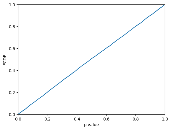
Norm CPS
KS-test: 0.5444229022986096

Mond CPS
KS-test: 0.5731223246624859

Mond norm CPS
KS-test: 0.5636493817142323

Similarly, we can obtain prediction intervals using online calibration:
[134]:
cps_std.predict_int(X_test, y_test, online=True)
[134]:
array([[-0.00395855, 0.05635648],
[ 0.03865984, 0.09897487],
[ 0.03711705, 0.09743208],
...,
[ 0.15147203, 0.21307479],
[-0.00933412, 0.05226863],
[ 0.0484321 , 0.11003486]])
[135]:
cps_norm.predict_int(X_test, y_test, online=True)
[135]:
array([[0.01412503, 0.03313546],
[0.02630808, 0.10380777],
[0.0435523 , 0.08494796],
...,
[0.11896677, 0.2409256 ],
[0.0135436 , 0.02600575],
[0.05903926, 0.09573046]])
[136]:
cps_mond_std.predict_int(X_test, y_test, online=True)
[136]:
array([[0.01171055, 0.0359984 ],
[0.03912007, 0.09068248],
[0.03757728, 0.08913969],
...,
[0.1169922 , 0.26185688],
[0.00778157, 0.03124527],
[0.05153735, 0.10433533]])
[137]:
cps_mond_norm.predict_int(X_test, y_test, online=True)
[137]:
array([[0.01149596, 0.03400184],
[0.02888577, 0.09760103],
[0.04492915, 0.08163269],
...,
[0.11601287, 0.25353761],
[0.0125025 , 0.02613013],
[0.05977328, 0.09504222]])
We can also get (lower and higher) percentiles using online calibration:
[138]:
cps_std.predict_percentiles(X_test, y_test,
lower_percentiles = [2.5, 25],
higher_percentiles = [50, 75, 97.5],
y_min=0, y_max=1, online=True)
[138]:
array([[0. , 0.01818573, 0.0234039 , 0.02847676, 0.05635648],
[0.03865984, 0.06083424, 0.06601597, 0.0710886 , 0.09897487],
[0.03711705, 0.05926132, 0.06447318, 0.06954581, 0.09743208],
...,
[0.15147203, 0.17473267, 0.18020303, 0.18518411, 0.21307479],
[0. , 0.01392652, 0.01939214, 0.02437404, 0.05226863],
[0.0484321 , 0.071692 , 0.07715837, 0.08214026, 0.11003486]])
[139]:
cps_norm.predict_percentiles(X_test, y_test,
lower_percentiles = [2.5, 25],
higher_percentiles = [50, 75, 97.5],
y_min=0, y_max=1, online=True)
[139]:
array([[0.01412503, 0.02142094, 0.02376185, 0.02597706, 0.03313546],
[0.02630808, 0.05605126, 0.06558458, 0.07462459, 0.10380777],
[0.0435523 , 0.05942572, 0.06453144, 0.06936007, 0.08494796],
...,
[0.11896677, 0.16404656, 0.17933112, 0.19385401, 0.2409256 ],
[0.0135436 , 0.01815 , 0.01971074, 0.02119576, 0.02600575],
[0.05903926, 0.07262089, 0.07721259, 0.08158103, 0.09573046]])
[140]:
cps_mond_std.predict_percentiles(X_test, y_test,
lower_percentiles = [2.5, 25],
higher_percentiles = [50, 75, 97.5],
y_min=0, y_max=1, online=True)
[140]:
array([[0.01171055, 0.02031295, 0.02372605, 0.02663451, 0.0359984 ],
[0.03912007, 0.0595464 , 0.06599388, 0.07316745, 0.09068248],
[0.03757728, 0.05797273, 0.06440488, 0.07162466, 0.08913969],
...,
[0.1169922 , 0.16694858, 0.17892996, 0.19135335, 0.26185688],
[0.00778157, 0.01650279, 0.0199145 , 0.02278111, 0.03124527],
[0.05153735, 0.07003037, 0.07691832, 0.08398725, 0.10433533]])
[141]:
cps_mond_norm.predict_percentiles(X_test, y_test,
lower_percentiles = [2.5, 25],
higher_percentiles = [50, 75, 97.5],
y_min=0, y_max=1, online=True)
[141]:
array([[0.01149596, 0.02079434, 0.02385006, 0.02619355, 0.03400184],
[0.02888577, 0.05720281, 0.06575971, 0.07580131, 0.09760103],
[0.04492915, 0.06004087, 0.06461938, 0.0699886 , 0.08163269],
...,
[0.11601287, 0.16203996, 0.17811182, 0.19510569, 0.25353761],
[0.0125025 , 0.01794109, 0.01988931, 0.02142942, 0.02613013],
[0.05977328, 0.07270317, 0.07718934, 0.08164919, 0.09504222]])
We can also obtain the full conformal predictive distributions (cpds) using online calibration. For standard and normalized conformal predictive systems, each cpd will contain one more value than the preceding, since the calibration set is growing by one element for each prediction.
[142]:
cpds = cps_norm.predict_cpds(X_test, y_test, online=True)
plt.plot(np.arange(len(cpds)), [len(cpds[i]) for i in range(len(cpds))])
plt.xlabel("#test objects")
plt.ylabel("calibration set size")
plt.ylim(0)
plt.xlim(0)
plt.show()
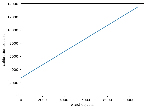
For Mondrian conformal predictive systems, the calibration set for one of the categories will be extended with one element for each prediction; the size of the predicted cpd is dependent on which category the test object falls in.
[143]:
cpds = cps_mond_norm.predict_cpds(X_test, y_test, online=True)
plt.plot(np.arange(len(cpds)), [len(cpds[i]) for i in range(len(cpds))])
plt.xlabel("#test objects")
plt.ylabel("calibration set size")
plt.ylim(0)
plt.xlim(0)
plt.show()
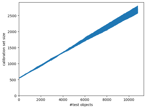
By default, the test objects and labels are sequentially added to the existing calibration set, i.e., the one used when fitting the conformal regressor. We may set the warm_start option to False, if we would like to ignore the original calibration set. Note that the initial predictions tend to be very (maximally) wide, before we have a sufficiently large calibration set to allow for providing tighter intervals at the specified level of confidence.
[144]:
cps_std.predict_int(X_test, y_test, online=True, warm_start=False)
[144]:
array([[ -inf, inf],
[ -inf, inf],
[ -inf, inf],
...,
[ 0.15104666, 0.21324685],
[-0.00975949, 0.0524407 ],
[ 0.04800673, 0.11020692]])
[145]:
cps_norm.predict_int(X_test, y_test, online=True, warm_start=False)
[145]:
array([[ -inf, inf],
[ -inf, inf],
[ -inf, inf],
...,
[0.11903777, 0.24105482],
[0.01355085, 0.02601895],
[0.05909007, 0.0957693 ]])
[146]:
cps_mond_std.predict_int(X_test, y_test, online=True, warm_start=False)
[146]:
array([[ -inf, inf],
[ -inf, inf],
[ -inf, inf],
...,
[0.11831232, 0.26189358],
[0.00778212, 0.03072091],
[0.05201278, 0.10533728]])
[147]:
cps_mond_norm.predict_int(X_test, y_test, online=True, warm_start=False)
[147]:
array([[ -inf, inf],
[ -inf, inf],
[ -inf, inf],
...,
[0.11609057, 0.25317732],
[0.01284918, 0.02601695],
[0.05979758, 0.09565872]])
Similarly, we can request percentiles while disabling warm_start for online calibration:
[148]:
cps_std.predict_percentiles(X_test, y_test,
lower_percentiles = [2.5, 25],
higher_percentiles = [50, 75, 97.5],
y_min=0, y_max=1,
online=True, warm_start=False)
[148]:
array([[0. , 0. , 1. , 1. , 1. ],
[0. , 0. , 0.06188396, 1. , 1. ],
[0. , 0. , 0.06034117, 1. , 1. ],
...,
[0.15104666, 0.17470576, 0.18023206, 0.18522357, 0.21324685],
[0. , 0.01389285, 0.01942517, 0.02441741, 0.0524407 ],
[0.04800673, 0.07165353, 0.0771914 , 0.08218364, 0.11020692]])
When disabling warm_start, we can observe that size of the cpd (= size of the calibration set) is initially zero:
[149]:
cpds = cps_norm.predict_cpds(X_test, y_test, online=True, warm_start=False)
plt.plot(np.arange(len(cpds)), [len(cpds[i]) for i in range(len(cpds))])
plt.xlabel("#test objects")
plt.ylabel("calibration set size")
plt.ylim(0)
plt.xlim(0)
plt.show()
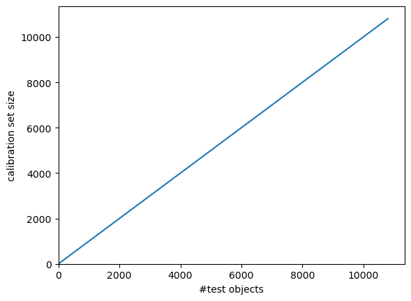
Similarly for Mondrian conformal predictive systems:
[150]:
cpds = cps_mond_norm.predict_cpds(X_test, y_test, online=True, warm_start=False)
plt.plot(np.arange(len(cpds)), [len(cpds[i]) for i in range(len(cpds))])
plt.xlabel("#test objects")
plt.ylabel("calibration set size")
plt.ylim(0)
plt.xlim(0)
plt.show()
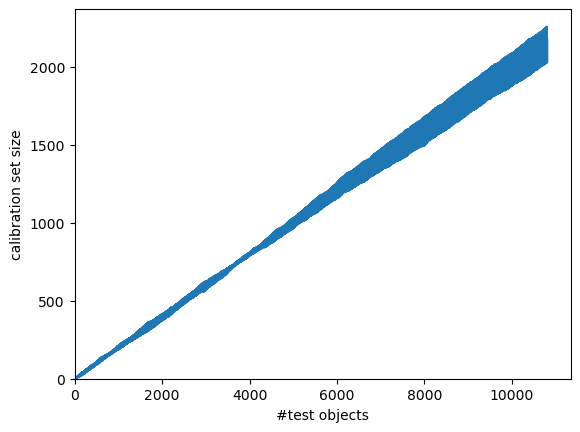
We may also evaluate the conformal predictive systems using online calibration, by specifying online=True for the evaluate method:
[151]:
cps_std.evaluate(X_test, y_test, confidence=0.99, y_min=0, y_max=1,
online=True)
[151]:
{'error': 0.009438327010271141,
'eff_mean': 0.13050333531919073,
'eff_med': 0.13328819829508187,
'time_fit': 0.00017309188842773438,
'ks_test': 0.5862834228370304,
'time_evaluate': 0.12139892578125}
[152]:
cps_norm.evaluate(X_test, y_test, confidence=0.99, y_min=0, y_max=1,
online=True)
[152]:
{'error': 0.010086055334505462,
'eff_mean': 0.09197006810319382,
'eff_med': 0.07304121558813316,
'time_fit': 4.363059997558594e-05,
'ks_test': 0.5593656069686399,
'time_evaluate': 0.12764263153076172}
[153]:
cps_mond_std.evaluate(X_test, y_test, confidence=0.99, y_min=0, y_max=1,
online=True)
[153]:
{'error': 0.008327935597298053,
'eff_mean': 0.10466048325746363,
'eff_med': 0.0727406751475411,
'time_fit': 0.0007212162017822266,
'ks_test': 0.617811678049804,
'time_evaluate': 0.07747888565063477}
[154]:
cps_mond_norm.evaluate(X_test, y_test, confidence=0.99, y_min=0, y_max=1,
online=True)
[154]:
{'error': 0.009808457481262134,
'eff_mean': 0.09613310447814595,
'eff_med': 0.0686948260683313,
'time_fit': 0.0006058216094970703,
'ks_test': 0.6106982217194512,
'time_evaluate': 0.08268046379089355}
Again, we may consider ignoring the original calibration set by setting warm_start=False:
[155]:
cps_mond_norm.evaluate(X_test, y_test, confidence=0.99, y_min=0, y_max=1,
online=True, warm_start=False)
[155]:
{'error': 0.00666234847783842,
'eff_mean': 0.1081167791835062,
'eff_med': 0.07772738299787259,
'time_fit': 0.0006058216094970703,
'CRPS': 0.006945326904468394,
'ks_test': 0.001502677422848499,
'time_evaluate': 0.35578370094299316}
Online calibration without an initial calibration set#
Since the calibration set is incrementally extended during online calibration, we may consider starting with an empty calibration set; this allows us to use the full training set when fitting the underlying model.
[156]:
rf_full = WrapRegressor(RandomForestRegressor(n_jobs=-1, n_estimators=500))
rf_full.fit(X_train, y_train)
Let us first initialize the conformal predictive system with an empty calibration set, i.e., not specifying any objects or labels for the calibrate method, but just setting cps=True (as we will see further below, we may additionally provide parameters such as difficulty estimator, Mondrian categorizer, etc.):
[157]:
rf_full.calibrate(cps=True)
[157]:
WrapRegressor(learner=RandomForestRegressor(n_estimators=500, n_jobs=-1), calibrated=False)
We may now obtain prediction intervals while sequentially updating the calibration set:
[158]:
rf_full.predict_int(X_test, y_test, confidence=0.9, online=True)
[158]:
array([[ -inf, inf],
[ -inf, inf],
[ -inf, inf],
...,
[ 0.16297635, 0.20348563],
[-0.00128962, 0.0392275 ],
[ 0.05723229, 0.09774942]])
Let us investigate also the p-values:
[159]:
p_values = rf_full.predict_p(X_test, y_test, online=True)
display(p_values)
plt.ecdf(p_values)
plt.xlim(0,1)
plt.xlabel("p-value")
plt.ylabel("ECDF")
plt.show()
print(f"KS-test: {kstest(p_values, "uniform").pvalue}")
array([0.1428238 , 0.5259196 , 0.41479209, ..., 0.96655256, 0.86741389,
0.34168146])

KS-test: 0.5860921941841599
If we provide also a difficulty estimator to calibrate, we will obtain a normalized conformal predictive system:
[160]:
de_var = DifficultyEstimator()
de_var.fit(X=X_train, learner=rf_full.learner, scaler=True)
rf_full.calibrate(de=de_var, cps=True)
[160]:
WrapRegressor(learner=RandomForestRegressor(n_estimators=500, n_jobs=-1), calibrated=False)
Now we get the intervals in the usual way:
[161]:
rf_full.predict_int(X_test, y_test, confidence=0.9, online=True)
[161]:
array([[ -inf, inf],
[ -inf, inf],
[ -inf, inf],
...,
[0.10048428, 0.26989887],
[0.00523275, 0.03377607],
[0.06200746, 0.09411756]])
Let us investigate also the p-values:
[162]:
p_values = rf_full.predict_p(X_test, y_test, online=True)
display(p_values)
plt.ecdf(p_values)
plt.xlim(0,1)
plt.xlabel("p-value")
plt.ylabel("ECDF")
plt.show()
print(f"KS-test: {kstest(p_values, "uniform").pvalue}")
array([0.10247823, 0.76073051, 0.65005368, ..., 0.71636374, 0.91023675,
0.34649296])

KS-test: 0.693509239808671
We get a Mondrian conformal predictive system by providing a Mondrian categorizer to calibrate:
[163]:
mc = MondrianCategorizer()
mc.fit(X_cal, de=de_var, no_bins=10)
rf_full.calibrate(mc=mc, cps=True)
[163]:
WrapRegressor(learner=RandomForestRegressor(n_estimators=500, n_jobs=-1), calibrated=False)
We use the same call again to get the intervals from the Mondrian conformal predictive system:
[164]:
rf_full.predict_int(X_test, y_test, confidence=0.9, online=True)
[164]:
array([[ -inf, inf],
[ -inf, inf],
[ -inf, inf],
...,
[0.13435379, 0.24302711],
[0.00981743, 0.02825416],
[0.05607963, 0.10150719]])
Let us investigate the coverage and prediction interval size for each category (here limiting the lower and upper bounds of the intervals):
[165]:
prediction_intervals = rf_full.predict_int(X_test, y_test, y_min=0,
y_max=1, confidence=0.99,
online=True)
number = []
coverage = []
size = []
bins_test = mc.apply(X_test)
for c in range(len(mc.bin_thresholds)-1):
selection = bins_test == c
number.append(np.sum(selection))
coverage.append(np.sum(
(prediction_intervals[selection,0] <= y_test[selection])& \
(y_test[selection] <= prediction_intervals[selection,1]))/np.sum(selection))
size.append(np.sum(prediction_intervals[selection,1]-\
prediction_intervals[selection,0])/np.sum(selection))
df = pd.DataFrame({"Number":number, "Coverage":coverage, "Size":size})
df.round(4)
[165]:
| Number | Coverage | Size | |
|---|---|---|---|
| 0 | 138 | 1.0000 | 1.0000 |
| 1 | 467 | 0.9936 | 0.4391 |
| 2 | 664 | 0.9940 | 0.3245 |
| 3 | 742 | 0.9892 | 0.2950 |
| 4 | 959 | 0.9927 | 0.2334 |
| 5 | 1089 | 0.9954 | 0.2244 |
| 6 | 1192 | 0.9941 | 0.2087 |
| 7 | 1851 | 0.9908 | 0.1714 |
| 8 | 1897 | 0.9921 | 0.1850 |
| 9 | 1808 | 0.9923 | 0.3287 |
Let us investigate also the p-values:
[166]:
p_values = rf_full.predict_p(X_test, y_test, online=True)
display(p_values)
plt.ecdf(p_values)
plt.xlim(0,1)
plt.xlabel("p-value")
plt.ylabel("ECDF")
plt.show()
print(f"KS-test: {kstest(p_values, "uniform").pvalue}")
array([0.11352531, 0.1064683 , 0.45958984, ..., 0.83782045, 0.9645613 ,
0.37016207])

KS-test: 0.21939702785457305
Similarly, we can also request percentiles using online calibration:
[167]:
rf_full.predict_percentiles(X_test, y_test,
lower_percentiles = [2.5, 25],
higher_percentiles = [50, 75, 97.5],
y_min=0, y_max=1, online=True)
[167]:
array([[0. , 0. , 1. , 1. , 1. ],
[0. , 0. , 1. , 1. , 1. ],
[0. , 0. , 0.04151614, 1. , 1. ],
...,
[0.1240431 , 0.16571835, 0.18033758, 0.19698534, 0.26562317],
[0.00669698, 0.01570988, 0.01917435, 0.02261172, 0.03038097],
[0.05175739, 0.06883639, 0.07629666, 0.08460016, 0.10687744]])
We can of course also request the cpds; here we take a close look at those belonging to category 5:
[168]:
cpds = rf_full.predict_cpds(X_test, y_test, online=True)
cpds[bins_test == 5]
[168]:
array([array([], dtype=float64), array([0.01216602]),
array([0.02279715, 0.0242049 ]), ...,
array([-0.02495182, -0.01059043, -0.0099913 , ..., 0.04228037,
0.04246528, 0.04585405]) ,
array([0.01532834, 0.02968973, 0.03028886, ..., 0.08256053, 0.08274544,
0.08613421]) ,
array([-0.00536258, 0.00899881, 0.00959793, ..., 0.06186961,
0.06205452, 0.06544329]) ],
dtype=object)
We may also evaluate the conformal predictive system using online calibration, by specifying online=True for the evaluate method:
[169]:
rf_full.evaluate(X_test, y_test, confidence=0.99, y_min=0, y_max=1, online=True)
[169]:
{'error': 0.007402609419820516,
'eff_mean': 0.2550916773218815,
'eff_med': 0.0754914906229507,
'time_fit': 6.4373016357421875e-06,
'ks_test': 0.6077975502348261,
'time_evaluate': 0.06209707260131836}